Download
1 / 34
340 likes | 476 Views
4DVar Assimilation (physics) in ROMS ESPreSSO * John Wilkin, Julia Levin, Javier Zavala-Garay. 2006 reanalysis (SW06) Operational system for OOI CI OSSE (ongoing)

E N D
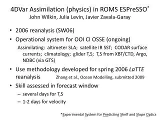
4DVar Assimilation (physics) in ROMS ESPreSSO*John Wilkin, Julia Levin, Javier Zavala-Garay • 2006 reanalysis (SW06) • Operational system for OOI CI OSSE (ongoing) Assimilating: altimeter SLA; satellite IR SST; CODAR surface currents; climatology; glider T,S; T,S from XBT/CTD, Argo, NDBC (via GTS) • Use methodology developed for spring 2006 LaTTE reanalysis Zhang et al., Ocean Modelling, submitted 2009 • Skill assessed in forecast window • several days for T,S • 1-2 days for velocity *Experimental System for Predicting Shelf and Slope Optics
ROMS ESPreSSO configuration • 5 km horizontal resolution Cape Cod to Cape Hatteras • 36 levels in traditional ROMS s-coordinate (stretching=1) • 4th order Akima T,S advection; 3rd order upwind u,v advection • Bathymetry, land-sea mask from NGDC Coastal Relief Model • Open boundary data HyCOM+NCODA (no bias correction) • stiff boundary nudging in forward simulations • Meteorology forcing 3-hourly 12-km NCEP NAM-WRF • 72-hour forecast window • sea level atmospheric conditions + bulk formulae = fluxes • [use NCEP NARR in 2006 reanalysis] • River daily average discharge USGS gauges • adjusted for ungauged fraction of watershed • Tides TPXO0.7 tides (5 harmonics) We are working in a data rich location for 4DVar assimilation…
Mid-Atlantic Regional Coastal Ocean Observing System (MARCOOS)CODAR, gliders, moorings, tide gauges, drifters, satellites …
IS4DVAR* • Given a first guess (the forward trajectory)… • and given the available data… *Incremental Strong Constraint 4-Dimensional Variational data assimilation
IS4DVAR • Given a first guess (the forward trajectory)… • and given the available data… • what change (or increment) to the initial conditions (IC) produces a new forward trajectory that better fits the observations?
The “best fit” becomes the analysis assimilation window ti = analysis initial time tf = analysis final time The strong constraintrequires the trajectory satisfies the physics in ROMS. The Adjoint enforces the consistency among state variables.
The final analysis state becomes the IC for the forecast window assimilation window forecast tf = analysis final time tf + t = forecast horizon
Forecast verification is with respect to data not yet assimilated assimilation window forecast verification tf + t = forecast horizon
LaTTE 2006 reanalysis (60 days) LaTTE domain and observation locations. Bathymetry of the New York Bight is in grayscale and dashed contours. yellow star is location of Ambrose Tower green squares are CODAR HF Radar sites
LaTTE 2006 reanalysis (60 days) Comparison of observed and modeled sea surface temperature and current at 0700 UTC 20 April 2006.
LaTTE 2006 reanalysis (60 days) 2-D histograms comparing observed and modeled temperature, salinity, and u-component of velocity model before (control simulation) and after (analysis) data assimilation. Color indicates the log10 of the number of observations.
Ensemble average of the DA skill for analysis and forecast periods for different data withheld from systemVertical bars are 95% confidence.Vertical dashed line is boundary between analysis and forecast. LaTTE 2006 reanalysis (60 days) Removing any data from the analysis system has more or less predictable negative impact on the forecast. More data is always better.
LaTTE 2006 reanalysis (60 days) • Ensemble average of the DA skill for analysis and forecast periods for different data withheld from system, evaluated with respect to: • glider-measured temperature and • satellite-measured SST Vertical bars are 95% confidence.Vertical dashed line is boundary between analysis and forecast. Satellite SST is crucial to forecast skill for this skill metric; namely, comparison to new observations in the forecast window.
4DVar Assimilation (physics) in ROMS ESPreSSO • 2006 reanalysis (SW06) • Basis for experiments with ecosystem and bio-optical modeling • 2009- operational System for OOI CI OSSE (ongoing) • 72-hour forecast (NAM-WRF meteorology) • tides, rivers, OBC HyCOM NCODA etc. • assimilates: • altimeter along-track SLA • satellite IR SST • CODAR surface currents • climatology • glider T,S • GTS: XBT/CTD, Argo, NDBC
Work flow for operational ESPreSSO/MARCOOS 4DVar Analysis interval is 00:00 – 24:00 UTC Input data preparation commences 01:00 EST (05:00 UT) • RU CODAR is hourly - but with 4-hour delay • RU glider T,S where available (approx 1 hour delay) • USGS daily average flow available 11:00 EST • persist in forecast • AVHRR IR passes (approx 2 hour delay) • HyCOM NCODA forecast updated daily • Jason-2 along-track SLA via RADS (4 to 16 hour delay) • GTS XBT/CTD, Argo, NDBC from AOML (intermittent) • T,S climatology (MOCHA)
Work flow for operational ESPreSSO/MARCOOS 4DVar Input preprocessing • RU CODAR de-tided (harmonic analysis) and binned to 5km • variance within bins and OI combiner expected u_err used for QC • ROMS tide solution added to de-tided CODAR – this approach reduces tide phase error contribution to cost function • RU glider T,S averaged to ~5 km horiz. and 5 m vertical bins • developed thermal lag salinity correction using constrained parametric fit to minimize statically unstable profiles • AVHRR IR individual passes 6-8 per day • use Matt Oliver’s cloud mask; bin to 5 km resolution • [2006 reanalysis uses REMSS daily SST OI combination of AVHRR, GOES, AMSR] • Jason-2 alongtrack 5 km bins (no coastal corrections) • MDT from 4DVAR on “mean model” (climatology 3D T,S, usurface, τwind)
Comparison of HF Radar observed and modeled M2 tide in LaTTE.
Work flow for operational ESPreSSO/MARCOOS • Input preprocessing completes approximately 05:00 EST • 4DVAR analysis completes approx 08:00 EST • 24-hour analysis is followed by 72-hour forecast using NCEP NAM 00Z cycle available from NOMADS OPeNDAP at 02:30 UT (10:30 pm EST) • Forecast complete and transferred to OPeNDAP by 09:00 EST • Effective forecast is ~ 60 hours OPeNDAP http://tashtego.marine.rutgers.edu:8080/thredds/catalog.html ncWMS http://tashtego.marine.rutgers.edu:8081/ncWMS/godiva2.html
Output OPeNDAP http://tashtego.marine.rutgers.edu:8080/thredds/catalog.html ncWMS http://tashtego.marine.rutgers.edu:8081/ncWMS/godiva2.html
Lessons from operational IS4DVAR for ESPreSSO • More and diverse data is better • use all available observations and platforms • Quality control • outliers in CODAR • cloud clearing from IR • coastal altimetry • High resolution regional climatology • removes bias from Open Boundary Condition • improves representation of dynamic modes and adjoint-based increments • IR SST individual passes work best with 4DVAR • time variability is explicitly resolved • implications for optics • Useful skill for operational applications • glider reachability forecast • Physics analysis affects ecosystem/optics model skill
Small scales may be important to large scale dynamics (and ecosystem) RU Endurance Line glider transect May 18-24, 2006
assimilation window tf = analysis final time
high-res assimilationwindow The analysis final hours becomes the data for the high-res 4DVAR, then forecast high-res forecast tf + t = forecast horizon assimilation window tf = analysis final time
Issues/Tasks ahead for 4DVAR ESPreSSO • High frequencies • Filter inertial oscillations/tides in increment when updating outer loop • High frequencies in coastal altimetry (keep or remove IB correction?) • Background error covariance • Can we use multi-variate “balance” constraint in coastal ocean? • Wide shelf, steep slope, anisotropic variability • Ecosystem / bio-optics? • Ecosystem/bio-optics assimilation in 4DVar • have Adjoint for NZPD model (ecosystem emphasis) • have Adjoint for simple bio-optical model (IOP emphasis) • Climatology? Initialization? • need dense data set for assimilation development • twin experiments? • optics in Community Sediment Transport Model? • Couple ecosystem/optics with thermodynamics • interaction is significant on NJ inner shelf (“just do it”) • Downscaling • 1 km resolution grid (better bathymetry and land/sea mask) • 5 km IS4DVAR analysis at end of interval treated as “data” • assimilate analysis into 1 km model with 1 4DVAR cycle