Download
1 / 15
150 likes | 299 Views
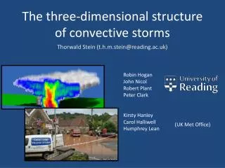
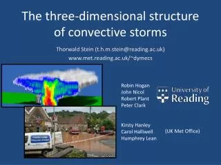
Thorwald Stein (t.h.m.stein@reading.ac.uk) www.met.reading.ac.uk/~dymecs. The three-dimensional structure of convective storms. Robin Hogan John Nicol Robert Plant Peter Clark Kirsty Hanley Carol Halliwell Humphrey Lean. (UK Met Office).

E N D
Thorwald Stein (t.h.m.stein@reading.ac.uk) www.met.reading.ac.uk/~dymecs The three-dimensional structure of convective storms Robin Hogan John Nicol Robert Plant Peter Clark Kirsty Hanley Carol Halliwell Humphrey Lean (UK Met Office)
NWP models run at km-scale: errors in timing, location, structure of convective precipitation. • Storm analysis of 2D fields (surface rainfall rate, OLR) highlights errors, but not underlying processes. • Use high-resolution (300m) radar observations for many storms to evaluate model storm morphology and dynamics. The three-dimensional structure of convective storms
The three-dimensional structure of convective storms UKV 1500m 200m Animations by Robin Hogan
The DYMECS approach: beyond case studies Track storms in real time and automatically scan Chilbolton radar • Derive properties of hundreds of storms on ~40 days: • Vertical velocity • 3D structure • Rain & hail • Ice water content • TKE & dissipation rate Met Office 1km rainfall composite 25m diameter S-band (3 GHz) Steerable (2 degrees per second) 0 dBZ out to 150 km • Evaluate these properties in model varying: • Resolution • Microphysics scheme • Sub-grid turbulence parametrization
40 dBZ • 20 dBZ • 0 dBZ Storm structure from radar Radar reflectivity (dBZ) Distance north (km) Distance east (km)
Median storm diameter with height “Convergence”? Observations UKV 1500m 500m 200m Drizzle from nowhere? “Shallow” Lack of anvils? “Deep”
Vertical profiles ofreflectivity Model: High rainfall rate from storms lacking ice or have ice cloud dBZ<0 Conditioned on average reflectivity at 200-1000m below 0oC. Reflectivity distributions forprofiles with thismean Z 40-45 dBZ are shown. 1.5-km + graupel 1.5-km Observations 200-m 1.5-km no crystals
Interquartile rangerain dBZconditioned onice dBZ Model: For ice dBZ < 20 Top 50% of rain dBZare 5-10 dB too high No crystals?Aggregates-onlyrain dBZ 5-10 dBtoo low.
Chapman & Browning (1998) • In quasi-2D features (e.g. squall lines) can assume continuity to estimate vertical velocity Updrafts? • Hogan et al. (2008) • Track features in radial velocity from scan to scan
Updraft retrieval Observations UKV 1500m Reflectivity 40 dBZ Estimated vertical velocity +10 m/s Estimate vertical velocity from vertical profiles of radial velocity, assuming zero divergence across plane. -10 m/s 10 km height Actual model vertical velocity Quantify errors due to 2D flow assumption 20 km width (slide courtesy John Nicol)
Vertical velocity distributions with height Observations 500m Estimated vertical velocity down up down up 2. Use map to simulate “true” observed PDF 1. Derive map from PDF of estimates to PDF of true model velocities True vertical velocity down up (slide courtesy John Nicol) Radar data with dBZ>0 within 90 km of the radar
Vertical velocity distribution between 7-8 km True model velocity Estimated model velocity Radar estimated velocity Radar mapped “true” velocity 500m simulation compares well with radar using 2D flow assumption (dashed lines) map (slide courtesy John Nicol)
Evaluation of width of updrafts • Retrieval in both observations and model: • wmin=0.5 m/s; wmax>3.0m/s • True model versus mapped observations: • wmin=1.0 m/s; wmax>5.0m/s • Model updrafts shrink with resolution • 200-m model has about the right width • Does 100-m model shrink further or stay the same? • How does Smagorinsky mixing length affect model? Observations 200-m model 500-m model 1.5-km model
Thorwald Stein (t.h.m.stein@reading.ac.uk) www.met.reading.ac.uk/~dymecs The three-dimensional structure of convective storms Models with smaller grid length producenarrower storms, similar to observations. Models associate shallow ice cloudwith high rainfall too frequently. 500m grid length model has verticalvelocity distribution comparable toobservations. Future work: Study the “E” of DYMECS.
Mixing-length sensitivityin 200m storm structures 40m mixing length 100m mixing length 300m mixing length 500m model 1500m model 200m simulation can approximate storm structures in coarser grid-length simulations by varying mixing length