Download
1 / 38
390 likes | 593 Views
Simulation of psk -based digital transmission schemes. Presented by: Group 2. Phase-Shift Keying (PSK). Two-level PSK (BPSK) Uses two phases to represent binary digits Where we can consider the above two functions to be multiplied by +1 and -1 for a binary 1 and binary 0 respectively.

E N D
Simulation of psk-based digital transmission schemes Presented by: Group 2
Phase-Shift Keying (PSK) • Two-level PSK (BPSK) • Uses two phases to represent binary digits Where we can consider the above two functions to be multiplied by +1 and -1 for a binary 1 and binary 0 respectively which equals
Phase-Shift Keying (PSK) • Differential PSK (DPSK) • Phase shift with reference to previous bit • Binary 0 – signal burst of same phase as previous signal burst • Binary 1 – signal burst of opposite phase to previous signal burst • The term differential is used because the phase shift is with reference to the previous bit • Doesn’t require an accurate receiver oscillator matched with the transmitter for the phase information but obviously depends to the preceding phase (information bit) being received correctly.
Phase-Shift Keying (PSK) • Four-level PSK (QPSK - quadrature PSK) • Each element represents more than one bit
QPSK and OQPSK Modulators I stream (in-phase) Q stream (quadrature data stream)
OQPSK (Offset QPSK) • OQPSK has phase transitions between every half-bit time that never exceeds 90 degrees (π/2 radians) • Results in much less amplitude variation of the bandwidth-limited carrier • BER is the same as QPSK • When amplified, QPSK results in significant bandwidth expansion, whereas OQPSK has much less bandwidth expansion especially if the channel has non-linear components
Multiple Level PSK amplitude and phase • Multilevel PSK • Using multiple phase angles with each angle having more than one amplitude, multiple signals elements can be achieved • D = modulation rate, baud • R = data rate, bps (note the difference in baud and bps) • M = number of different signal elements = 2L • L = number of bits per signal element • If L = 4 bits in each signal element using M = 16 combinations of amplitude and phase, then if the data rate is 9600 bps,the line signaling speed/modulation rate is 2400 baud
Quadrature Amplitude Modulation • QAM is a combination of ASK and PSK • Two different signals sent simultaneously on the same carrier frequency
MATLAB Resutls • Program 3.2 (bpsk_fading)
Output – Flat Fading Channel(Amplitude Distortion)Rolloff Factor = [0 0.5 1]
Received Constellation Amplitude + Phase Distortion Amplitude Distortion
Nyquist Pulses Input sr=256000.0; % Symbol rate ipoint=2^03; % Number of oversamples ncc=1; %******************* Filter initialization ******************** irfn=21; % Number of filter taps
Plot of data1 • Number of symbols (nd) = 10 • data=rand(1,nd)>0.5 • data1=data.*2-1
Plot of data2 • [data2] = oversamp( data1, nd , IPOINT)
Plot of data3 • data3 = conv(data2,xh)
BPSK Demodulation • demodata=data6 > 0
Eye diagram Source: Wikipedia • Graphical eye pattern showing an example of two power levels in an OOK modulation scheme. Constant binary 1 and 0 levels are shown, as well as transistions from 0 to 1, 1 to 0, 0 to 1 to 0, and 1 to 0 to 1
MSK – Minimum Shift Keying • MSK is a continuous phase FSK (CPFSK) where the frequency changes occur at the carrier zero crossings. • MSK is unique due to the relationship between the frequency of a logic 0 and 1. • The difference between the frequencies is always ½ the data rate. • This is the minimum frequency spacing that allows 2 FSK signals to be coherently orthogonal.
MSK – How It Works • The baseband modulation starts with a bitstream of 0’s and 1’s and a bit-clock. • The baseband signal is generated by first transforming the 0/1 encoded bits into -1/1 using an NRZ filter. • This signal is then frequency modulated to produce the complete MSK signal. • The amount of overlap that occurs between bits will contribute to the inter-symbol interference (ISI).
Example of MSK • 1200 bits/sec baseband MSK data signal • Frequency spacing = 600Hz a) NRZ data b) MSK signal
Pros of MSK • Since the MSK signals are orthogonal and minimal distance, the spectrum can be more compact. • The detection scheme can take advantage of the orthogonal characteristics. • Low ISI (compared to GMSK)
Cons of MSK • The fundamental problem with MSK is that the spectrum has side-lobes extending well above the data rate (See figure on next slide). • For wireless systems which require more efficient use of RF channel BW, it is necessary to reduce the energy of the upper side-lobes. • Solution – use a pre-modulation filter: • Straight-forward Approach: Low-Pass Filter • More Efficient/Realistic Approach: Gaussian Filter
The Need for GMSK • Gaussian Filter • Impulse response defined by a Gaussian Distribution – no overshoot or ringing (see lower figure) • BT – refers to the filter’s -3dB BW and data rate by: • Notice that a bit is spread over more than 1 bit period. This gives rise to ISI. • For BT=0.3, adjacent symbols will interfere with each other more than for BT=0.5 • GMSK with BT=∞ is equivalent to MSK. • Trade-off between ISI and side-lobe suppression (top and bottom figures) • The higher the ISI, the more difficult the detection will become.
GMSK – Applications • An important application of GMSK is GSM, which is a time-division multiple-access system. • For this application, the BT is standardized at 0.3, which provides the best compromise between increased bandwidth occupancy and resistance to ISI. • Ninety-nine percent of the RF power of GMSK signals is specified to confine to 250kHz (+/- 25kHz margin from the signal), which means that the sidelobes need to be virtually zero outside this frequency band and the ISI should be negligible.
Comments • The program bpsk.m prints the BER in each simulation loop, and this causes the program to run slowly, therefore, I stopped printing those results. Instead, I plotted the BER vs. EbN0 with a counter that displays the current value of EbN0. • I tried to plot the eye diagram for QPSK, but I didn’t succeed in that.
References • Wikepedia.com • Haykin, S. 2001: “Communication Systems”. 4th ed. New York, NY. John Wiley & Sons. • Introduction to GMSK www.eecs.tufts.edu/~gcolan01 • GMSK: Practical GMSK Data Transmission http://www.eetchina.com/ARTICLES/2003AUG/PDF/2003AUG29_NTEK_AN.PDF • Minimum Shift Keying: A Spectrally EffiecientModulation http://www.elet.polimi.it/upload/levantin/SistemiIntegrati/msk_pasupathy_1979.pdf