Download

1 / 44
520 likes | 1.06k Views
Coalescent theory. Expectation, and deviance. Statements such as the ones below can be made only if we have an underlying model that suggests what we should expect. Recombination rates vary dramatically across the genome There was a population bottleneck in Iceland

E N D
Coalescent theory Vineet Bafna
Expectation, and deviance • Statements such as the ones below can be made only if we have an underlying model that suggests what we should expect. • Recombination rates vary dramatically across the genome • There was a population bottleneck in Iceland • We would like models for populations. • Sometimes, even with a model, it is hard to compute expected values, etc. In this case, we resort to simulations. • We should be able to simulate populations. Vineet Bafna
Goal: simulating population data • Recall that a population sample can be thought of as a binary matrix. • Rows (n) are individuals. n<<N (population size) • Columns are variant sites. • Suppose you are given some parameters about a population (mutation rates, size, time of evolution). • Can you quickly generate a population with those parameters? • What is the model, and how much time would it take? Vineet Bafna
Wright Fisher Model of Evolution • Fixed population size from generation to generation • Random mating Vineet Bafna
WF model assumptions • Assumptions (implicit/explicit) • Discrete and non-overlapping generations • Constant population size (2N haplotypes) across generations • All individuals are equally fit. • No geographical or social structure. Random mating. • No recombination. Each haplotype is identical to its parent except at mutating positions. • We also make the infinite sites assumption. Vineet Bafna
Generating populations • Forward simulation for generating a population of n<<2N haplotypes: • Start with a population of 2N haplotypes (random binary strings) • Simulate genealogy for T generations • Drop mutation according to fixed rate , each at a new site. (Let m be the total number of mutations) • Generate haplotypes • Sample nhaplotypes • How much time will it take to generate a random population? O(NTm) • It turns out that this process can be accomplished in nm steps Vineet Bafna
Coalescent model • Insight 1: • Separate the genealogy from allelic states (mutations) • First generate the genealogy (who begat whom) Vineet Bafna
Coalescent theory • Insight 2: • Much of the genealogy is irrelevant, because it disappears. • Better to go backwards Vineet Bafna
Coalescent approximation • Insight 3: • Topology is independent of coalescent times • If you have n individuals, generate a random binary topology • Iterate (until one individual) • Pick a pair at random, and coalesce • Insight 4: • To generate coalescent times, there is no need to go back generation by generation Vineet Bafna
A brief digression on common distributions • Exponential distribution • Poisson distribution Vineet Bafna
The exponential distribution (discrete case) • Exponential: Consider the case of tossing coins until you first see HEADS. • Let Probability [Heads]=p, • Let q=1-p • Q: Number of steps to success? Vineet Bafna
Expectation Vineet Bafna
Poisson distribution • Ex: Throw darts at a line so that so that every unit interval has an average of λ darts. • P[k]=Pr[Interval has exactly k darts]? Vineet Bafna
Coalescent theory (Kingman) • Input • (Fixed population (N individuals), random mating) • Consider 2 individuals. • Probability that they coalesce in the previous generation (have the same parent)= • Probability that they do not coalesce after t generations= Vineet Bafna
Coalescent theory • is time in units of 2N generations • Consider k individuals. • Probability that no pair coalesces after 1 generation • Probability that no pair coalesces after t generations Vineet Bafna
Coalescent approximation • At any step, there are 1 <= k <= n individuals • To generate time to coalesce (k to k-1 individuals) • Pick a number from exponential distribution with rate k(k-1)/2 • Mean time to coalescence = 2/(k(k-1)) Vineet Bafna
Typical coalescents • 4 random examples with n=6 (Note that we do not need to specify N. Why?) • Expected time to coalesce? Vineet Bafna
Coalescent properties • Expected time for the last step • The last step is half of the total time to coalesce • Studying larger number of individuals does not change numbers tremendously • EX: Number of mutations in a population is proportional to the total branch length of the tree • E(Ttot) =1 Vineet Bafna
Coalescent properties • The time to MRCA is not sensitive to sample size • Pr[Sample of size n contains MRCA] • =(n-1)/(n+1) • A significant fraction of the SNPs are ‘ancient’ Vineet Bafna
Sample MRCA versus true MRCA • Proof sketch: • Let x be the fraction of individuals on the left side of the tree. • By symmetry, x is uniformly distributed in [0..1] (formal proof required) n N Vineet Bafna
Variants (exponentially growing populations) • If the population is growing exponentially, the branch lengths become similar, or even star-like. Why? • With appropriate scaling of time, the same process can be extended to various scenarios: male-female, hermaphrodite, segregation, migration, etc. Vineet Bafna
Simulating population data • Generate a coalescent (Topology + Branch lengths Vineet Bafna
Simulating population data • Generate a coalescent (Topology + Branch lengths) • For each branch length t, drop mutations with rate t • Based on infinite sites, each mutation is at a unique location 4 0 6,7 9 2,8 1,3,5 Vineet Bafna
Simulating population data • Generate Sequences 0 1 2 3 4 5 6 7 8 9 1 0 0 0 1 0 0 0 0 1 1 0 0 0 0 0 0 0 0 1 0 0 0 0 0 0 1 1 0 1 0 0 1 0 0 0 0 0 1 1 0 0 1 0 0 0 0 0 1 1 0 1 0 1 0 1 0 0 0 0 4 0 6,7 9 2,8 1,3,5 Vineet Bafna
Coalescent theory: example • Ex: ~1400bp at Sod locus in Dros. • 10 taxa • 5 were identical. The other 5 had 55 mutations. • Q: Is this a chance event, or is there selection for this haplotype. Vineet Bafna
Coalescent application • 10000 coalescent simulations were performed on 10 taxa. • 55 mutations on the coalescent branches • Count the number of times 5 lineages are identical • The event happened in 1.1% of the cases. • Conclusion: selection, or some other mechanism explains this data. Vineet Bafna
Coalescent example: Out of Africa hypothesis • Looking at lineage specific mutations might help discard the candelabra model. How? • How do we decide between the multi-regional and Out-of-Africa model? How do we decide if the ancestor was African? Vineet Bafna
Human Samples • We look at data from human samples • Gabriel et al. Science 2002. • 3 populations were sampled at multiple regions spanning the genome • 54 regions (Average size 250Kb) • SNP density 1 over 2Kb • 90 Individuals from Nigeria (Yoruban) • 93 Europeans • 42 Asian • 50 African American Vineet Bafna
Population specific recombination • D’ was used as the measure between SNP pairs. • SNP pairs were classified in one of the following • Strong LD • Strong evidence for recombination • Others (13% of cases) • Plot shows fraction of pairs with strong recombination (low LD) • This roughly favors out-of-africa. A Coalescent simulation can help give confidence values on this. Gabriel et al., Science 2002 Vineet Bafna
Coalescent theory applications • Coalescent simulations allow us to test various hypothesis. The coalescent/ARG is usually not inferred, unlike in phylogenies. Vineet Bafna
Coalescent theory Review • Under a specific model of evolution, coalescent theory allows us to simulate population data efficiently (linear in the size of the data). • This allows us to compute many summary statistics, and test hypotheses. Vineet Bafna
Coalescent with Recombination • An individual may have one parent, or 2 parents • The evolutionary history is not a tree, but an ancestral recombination graph (ARG) Vineet Bafna
ARG: Coalescent with recombination • Given: mutation rate , recombination rate r, population size 2N (diploid), sample size n. • How can you generate the ARG (topology+branch lengths) efficiently? • How will you generate sequences for n individuals? • Given sequence data, can you reconstruct the ARG (topology) Vineet Bafna
Recombination • Define r as the probability of recombining. • Note that the parameter is a scaled value which will be defined later • Assume k individuals in a generation. The following might happen: • An individual arises because of a recombination event between two individuals (It will have 2 parents). • Two individuals coalesce • Neither (Each individual has a distinct parent) • Multiple events (low probability) Vineet Bafna
Recombination • We ignore the case of multiple (> 1) events in one generation • Pr (No recombination) = 1-kr • Pr (No coalescence) • Consider scaled time in units of 2N generations. Thus the number of individuals increase with rate kr2N, and decrease with rate • The value 2rN is usually small, and therefore, the process will ultimately coalesce to a single individual (MRCA) Vineet Bafna
ARG • Let k = n, • Define • Iterate until k= 1 • Choose time from an exponential distribution with rate • Pick event as recombination with probability • If event is recombination, choose an individual to recombine, and a position, else choose a pair to coalesce. • Update k, and continue Vineet Bafna
Simulating sequences on an ARG • Simulate the ARG • Generate each of the constituent coalescents and revise mutation rates • Generate sequences for each of the coalescents • Concatenate Vineet Bafna
Recombination events and • Given , n, can you compute the expected number of recombination events? • It can be shown that E(n, ) = log (n) • The question that people are really interested in • Given a set of sequences from a population, compute the recombination rate • Given a population reconstruct the most likely history (as an ancestral recombination graph) • We will address this question in subsequent lectures Vineet Bafna
Estimating (scaled) mutation rate • Given a population sample evolving according to a coalescent without recombination, can you estimate μ(number of mutations per individual per generation)? • It is hard to estimate μ without additional information, but relatively easier to estimate scaled mutation rateθ=4Nμ 0 1 2 3 4 5 6 7 8 9 1 0 0 0 1 0 0 0 0 1 1 0 0 0 0 0 0 0 0 1 0 0 0 0 0 0 1 1 0 1 0 0 1 0 0 0 0 0 1 1 0 0 1 0 0 0 0 0 1 1 0 1 0 1 0 1 0 0 0 0 4 0 6,7 9 2,8 1,3,5 Vineet Bafna
Watterson’s estimate • Let S be the number of mutations in the history of a population sample. • If we make the infinite sites assumption, then S can be estimated • Recall that • E(Sn) =E(Ttot) • E(Sn) = 2N k 2/(k-1) = 4N ( + ln (n-1)) • Watterson’s estimate • W = Sn/ ( + ln (n-1)) Vineet Bafna
Tajima’s estimate of • Define ij = heterozygosity between two individuals • Note: heterozygosity = # differing sites = hamming distance i:0 1 0 0 0 0 1 1 0 j: 0 0 0 0 0 0 1 1 1 ij = 2 • Average heterozygosity can be empirically estimated from a sample as Vineet Bafna
Estimating Average heterozygosity • Assuming an underlying coalescent model of evolution, what is the average heterozygosity? • Q: Given 2 randomly picked individuals, what is the expected time to coalescence? • A: 2N • Q: Given 2 individuals what is the expected number of mutations in the lineages connecting them? • A: 2 2N = • Therefore, the average heterozygosity k is an estimate (Tajima’s estimate) of Vineet Bafna
Difference tests • Under neutral evolution, there are many different estimates of θ, all using coalescent theory. • You’ll explore these in homework 2. • If you take any two and take the difference, the expected value is 0. • Departure from neutrality is indicative of non-neutral evolution. Vineet Bafna
Coalescent theory: summary of results • CT can be used to efficiently generate populations • Test out possible departures from neutrality. • The theory also helps estimate various parameters of a population sample • Scaled mutation rate, θ • Effective population size, N • Time to MRCA (4N) • Likely genealogical history of the population sample (Perfect phylogeny, ancestral recombination graph) Vineet Bafna