Download
1 / 1
10 likes | 130 Views
Fig.1. Detector 3 – 9, natural weighting. Fig. 2. Detectors 3 – 9, uniform weighting. Fig. 3. Detectors 2 – 9, natural weighting. Fig. 4. Detector 1 – 9, natural weighting.

E N D
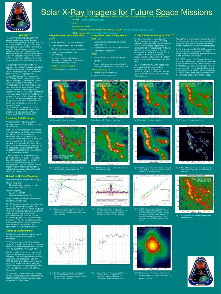
Fig.1. Detector 3 – 9, natural weighting Fig. 2. Detectors 3 – 9, uniform weighting. Fig. 3. Detectors 2 – 9, natural weighting. Fig. 4. Detector 1 – 9, natural weighting • Brian R. Dennis,1 Chau Dang, Mike Choi, George Voellmer, Larry White, Richard A. Schwartz,1,3 and A. Kimberley Tolbert1,4 • 1 Code 671 Brian.R.Dennis@nasa.gov • Code • 2 Oaklahoma State U. • 3 The Catholic University of America, Washington, DC 20064 richard.a.schwartz.1@gsfc.nasa.gov • 4 RSIS, Lanham, MD Anne.K.Tolbert.1@gsfc.nasa.gov ABSTRACT RHESSI X-ray imaging is possible with angular resolution as fine as 2 arcsec (FWHM) at energies from as low as 3 keV to >100 keV. However, taking full advantage of this capability has proven to be challenging given the Fourier-transform imaging technique that is used. In particular, it is difficult to image the finest source structures at the few arcsecond scale in the presence of Poisson noise and artifacts of the image reconstruction techniques that are available. In this poster, we show how judicious choices of the various free parameters of the CLEAN reconstruction procedure allow the source morphology to be best determined down to the most compact structures present. We illustrate the process with RHESSI and TRACE observations of the flare on 2005 May 13 reported by Liu et al. (2007). By taking full advantage of the RHESSI data from the finest grids, we can show that the hard X-ray emission comes from an extended range along the two ribbons seen with TRACE. This is in contrast to the usual case in which the hard X-rays are seen from only one or two points in each ribbon. This same imaging philosophy can be applied to other flares to determine the source size distribution down into the arcsecond range. Liu, C. and Lee, J. and Gary, D. E. and Wang, H., “The Ribbon-like Hard X-Ray Emission in a Sigmoidal Solar Active Region", ApJ., 658, L127-L130, 2007. • Image Reconstruction Algorithms • CLEAN • Quick evaluation of source morphology. • Same image details as other methods. • Defaults hide compact source structures. • ‘taper’ controls noise from finer subcollimators. • For finer resolution, use narrower Gaussian convolved with point source components found by CLEAN. • Uniform or natural weighting • Visibilities version in preparation • Image Reconstruction Algorithms • MEM_NJIT • Quick evaluation of source morphology. • Uses visibilities • Super-resolution with “best” subcollimators. • Over-resolution problem? • PIXON • Best photometry & lowest background • Very slow • Over-resolution problem controlled withPixon_resolution and/or pixon_sensitivity • Visibilities Forward Fit • For one or two sources only. • Best for source dimensions. 13 May 2005 Flare starting at 16:36 UT This flare has proven to be particularly informative about the quality of RHESSI images by comparison with cotemporaneous TRACE 1600 Å images. In particular, the optimized RHESSI images reveal hard X-ray emission from the full length of the two ribbons seen in the TRACE images. This is in contrast to the more usual isolated sources at a few locations along the ribbons that have been reported previously for other flares. Figs. 1 & 2 show the CLEAN images made with natural and uniform weighting, respectively, using the default set of subcollimators (3 to 8). This limits the finest source dimensions that can be resolved to ~10 arcseconds. Adding the two finest subcollimators in figures 3 and 4 shows that finer structure is present in the image but it is not clear if it is real or contains artifacts from the image reconstruction process. Overlaying contours of the RHESSI image from figure 4 onto the cotemporaneous TRACE image in figure 6 shows that all of the structures match above the 40% contour. The PIXON image in fig. 7 reveals the same structures seen in the CLEAN image shown with the same contour overlays. Note however, that the PIXON image shows broader, low intensity areas surrounding the two bright ribbons similar to that shown in the default CLEAN image in fig. 1. It is not clear if these features are real since they are not present in the TRACE image. Solar X-Ray Imagers for Future Space Missions Optimizing RHESSI Images All reconstruction techniques require subjective control of the data from the finest subcollimators. Each subcollimator produces a modulation of the corresponding detector counting rate only if there is source structure with dimensions equal to or finer than the resolution of that subcollimator. If there is no source structure with dimensions of less than say 10 arcseconds, then there will be no modulation of the counting rates through the finest grids. Including data from the corresponding detectors will only add noise to the reconstructed image. Currently, there is no automatic way to determine from the RHESSI counting rate data which subcollimators are producing significant modulation in the detector counting rates. Thus, the user must decide through trial and error which detectors to include in the analysis and how to weight them if they are included. Fig. 5. CLEAN images in three 20 s intervals. Shows little repeatability of smallest features. Fig. 6. TRACE 1600 Å image overlaid with contours of CLEAN image in fig. 4. Fig. 7. PIXON image overlaid with contours of CLEAN image in fig. 4. Shows same features but with lower PIXON background level. Fig. 8. MEM-NJIT image overlaid with contours of 25 to 50 keV image in fig. 4. Shows effects of over-resolution? Natural vs. Uniform Weighting Weighting schemes are illustrated in fig. 9. Natural weighting: All subcollimators weighted equally. Strong side lobes (fig. 10) Uniform weighting: Weight 1/FWHM Optimal side lobes (fig. 10) “Taper” allows exponential suppression of finest subcollimator data. Fig. 10 shows that the point spread function for uniform weighting has significantly smaller side lobes than for natural weighting. Thus, the combination of uniform weighting with a judicial choice of the “taper” parameter should produce the optimum CLEAN image. However, if the modulation amplitude for the finer subcollimators is low, using uniform weighting can result in the magnification of the noise and the appearance of false compact sources. Fig. 9. Weight given to each subcollimator for both natural and uniform weighting and for five different values of the “taper” parameter from 0 to 4 arcseconds. Fig. 10. Point spread functions for individual subcollimators and for all subcollimators with natural and uniform weighting. Note the smaller side lobes for uniform weighting. Fig.11. CLEAN’s default sigma of Gaussian used to display point-source components. Thus, if detectors 1 through 9 are chosen, the finest sources displayed will have a sigma of 2.5 arcsec (FWHM = 6 arcsec) even though detector # 1 has a FWHM resolution of 2.3 arcsec. Fig.12. CLEAN image with uniform weighting and a taper of 4 arcsec. Choice of Subcollimators To obtain the most detailed images, use all subcollimators that show significant modulation. For complex sources, visibility amplitudes can be <3 sigma for the finest subcollimators even though there is significant fine structure – see fig. 13 for the 13 May 2005 flare. Visibility amplitudes are good indicators of significant modulation for simple sources – see figure 14 for the single compact source seen at the limb for the flare on 20 April 2002. All visibility amplitudes are >3 sigma and Fig. 15 shows that uniform weighting can be used with all subcollimators included to reveal a compact source with a FWHM of 1.6 arcsec. For other flares, there is currently no recipe for making the best possible images showing all of the real fine structure. Various people are working on this problem. Fig. 13. Fractional visibility amplitudes plotted against the subcollimator (SC) number plus the positional angle. Note that most amplitudes for SC 6 and below are <3 sigma. Fig. 14. Same as fig 13 for flare on 20 April 2002 at 23:26 UT showing >3 sigma visibility amplitudes for all subcollimators. The corresponding image is shown in fig. 15. Fig.15. Smallest source ever imaged in hard X-rays. Uniform weighting, 0.2 arcsec pixels, taper = 0. FWHM = 1.6 arcsec.