4. IMAGE CLUSTERING

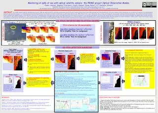
1. Monitoring oil spills at sea with optical satellite sensors: the PRIMI project Optical Observation ModulePisano, Andrea1 ; Bignami, Francesco1; Colella, Simone1; Evans, Robert, H.2; Santoleri, Rosalia1 1CNR-ISAC, Via Fosso del Cavaliere 100, 00133 Rome, Italy. e-mail: andrea.bignami@artov.isac.cnr.it; 2The Rosenstiel School of Marine and Atmospheric Science, 4600 Rickenbacker Causeway, Miami, FL 33149-1098, USA. e-mail: revans@rsmas.miami.edu ABSTRACT The PRIMI project funded by the Italian Space Agency (ASI) has implemented an observation and forecast system to monitor marine pollution from hydrocarbon oil spills (OS) in the Italian Seas. The system consists of four components, two of which for OS detection via multi-platform SAR and optical satellite imagery, an OS displacement forecast subsystem based on numerical circulation models and a central archive that provides WEB-GIS services to users. The system also provides meteorological, oceanographic and ship detection information. The Optical Observation Module, based on MODIS and MERIS imagery, is described here. The idea of combining wide swath optical observations with SAR monitoring arises from the necessity to overcome the SAR reduced coverage of the monitoring area. This can be done now, given the MODIS and MERIS higher spatial resolution with respect to older sensors (250-300 m vs. 1 km), which consents the identification of smaller spills deriving from illicit discharge at sea. The procedure to obtain identifiable spills in optical reflectance images involves removal of natural variability to enhance slick - clean water contrast, image segmentation/clustering and a set of criteria for the elimination of those features which look like spills (look-alikes). The final result is a classification of oil spill candidate regions by means of a score based on the above criteria. OIL SPILLS ARE DETECTABLE IN OPTICAL IMAGERY MERIS Imagery: L1B full resolution (300 m) TOA radiance bands: λ = (443, 560, 665, 681, 865 nm) MODIS Imagery: L1B high and medium resolution (250 and 500 m) TOA radiance bands: λ = (469, 555, 645, 859, 1240, 1640, 2130 nm) First criterion for OS detectability: High Glint Condition (specular reflection): OS is brighter than its background Low Glint Condition (no specluar reflection): OS is darker than its background t(469) t(645) t(555) High Glint Condition Low Glint Condition t(1240) t(2130) t(1640) t(859) t(443) t(865) t(681) t(560) t(665) MODIS TERRA true color image August 8, 2008 OS north of Algerian coast MERIS true color image, August 2, 2006, OS on Lebanon coast Striping effect OIL SPILL DETECTION ALGORITHM Input images: MODIS & MERIS L2 remapped TOA reflectance t() MODIS • DESTRIPING (MODIS only): • Eliminationof “striping” effect via • detector ramprectification & mirror side • Equalization • 2. CLOUD MASKING • (using SST qualityflags + cloudedgeexpansion) • 3. IMAGE FLATTENING • (eliminationofnaturalvariability) • Subtract Rayleigh reflectance r from t, all bands; • Subtract water-leaving reflectance (w) from t (MODIS:469, 555 nm only;MERIS: 443, 560 nmonly); • Subtract aerosol contribution using red band (645 nm). 5. OS CANDIDATE SELECTION Discard or retain cluster regions according to: Region Area (A): retain only regions within threshold values; Region Shape (S): computed combining A and perimeter P; (McGarigal and Marks 1995); retain only elongated regions; Region-water contrast (C=Region reflectance/water bbox reflectance): retain regions with C<1 (C>1) for low (high) glint cases; Cloud vicinity: elimination of regions made more brilliant by nearby cloud straylight, particularly important for high glint cases where brighter slicks may be confused with straylight affected regions Region and water reflectance histogram peak distance (dbe): retain regions with histogram peak reflectance sufficiently lower (higher) than surrounding water histogram peak reflectance for low (high) glint cases. Segmented images MERIS Flattened images () MODIS 4. IMAGE CLUSTERING Classification/grouping of ocean pixels, using mean shift segmentation (Comaniciu and Meer, 2002): image pixels are sorted out into clusters, each of which is defined by a reflectance mode value. MODIS MERIS MERIS 4 clusters • Each color  reflectance mode valuedefining a cluster • Each cluster composedbymanyregions • Reducedsignalvariabilityfrom input images • Stripingpartiallyremoved 3 clusters SCORE LOOK-UP TABLE (LUT) COMPUTATION the following parameters (P) are used to define scores (S) for OS candidates: dbe: see OS candidate selection; d4r: OS candidate reflectance histogram integral, from the minimum reflectance to a fourth of the reflectance total range (region + surrounding water) histograms; l4r: same as d4r, from 3/4 to the maximum reflectance of the above range; d4w and l4w: The same for the surrounding water reflectance histogram; (d4r – d4w)/max(d4r, d4w): This ratio is equal to 1 when the darkest quarter of the reflectance range is only populated by the OS candidate region histogram; no surrounding water in this range implies d4w = 0. Contrarily, the ratio is equal to -1 when only populated by surrounding water (thus, d4r = 0). In practice this parameter tells us how much more the darker range of the histogram is populated by the OS candidate than by water which means that, in the case of no glint conditions, then candidate is a probable oil spill; (l4r – l4w)/max(l4r, l4w):The same for the brighter quarter of the histogram reflectance range; values close to 1 in a high glint case probably indicate an OS; dref: Average reflectance distance between the OS candidate and water histogram integral curves; this parameter indicates how much an OS candidate region is “globally” darker or brighter than surrounding water. An “in situ certified”OS and look-alike database (64) was used as to compute score look-up tables (LUT), for each of the above parameters. Score table computation: Each of the above parameters was estimated for each OS or lookalike of our database. Histograms (H) of each parameter distribution were computed, both for known OS’s (HOS(P)) and look-alikes (HLA(P);) A score LUT for each parameter P was computed as S(P) = HOS(P)/(HOS(P)+ HLA(P)) . Candidate oil spills Output images • 6. SCORE ASSIGNMENT TO SELECTED OS CANDIDATES • For each selected OS candidate in a new image: • values P are computed for all score parameters; • Score values are found in each P LUT; • Final score is issued as a linear combination of single-P scores. MODIS MERIS score score The finalresultis a classificationof oil spill candidate regionsbymeansof a score (from 0 to 1) based on the abovecriteria Many regions are eliminated but OS are not yet inequivocably distinguishable from look-alikes MODIS MERIS REFERENCES Comaniciu and D., P. Meer, 2002. “Mean shift: a robust analysis of feature spaces: color image segmentation”. IEEE Trans. On pattern analysis and machine intelligence, 24, 5, 1-18. Gumley, L., R. Frey and C. Moeller, 2005. “Destriping of MODIS L1B 1KM Data for Collection 5 Atmosphere Algorithms”. http://modis.gsfc.nasa.gov/sci_team/meetings/200503/posters/atmos/gumley1.pdf. Weinreb, M. P., R. Xie, J. H. Lienesch and D. S. Crosby, 1989. “Destriping GOES Images by Matching Empirical Distribution Functions”. Remote Sens. Environ., 29, 185-195. McGarigal and Marks, 1995. “Spatial pattern analysis program for quantifying landscape structure”. http://www.umass.edu/landeco/pubs/mcgarigal.marks.1995.pdf • CONCLUSIONS AND FUTURE WORK • Imagedestriping, flattening (eliminationofoceanic and atmosphericnaturalvariabilityfrom the input • image), clustering and OS classification (bymeansof a set ofcriteria) are the basisof the OS detection • algorithmproposedhere. • It can beseenthat the end productstillpresentsambiguities in OS pinpointing, whichcallsfor future • work, towards a fullyautomatized OS detection Algorithm • Imagedestriping: notyetfullyperformant, requiresfutherdevelopment; • Score computation: ongoingrefinementof the score parameterswillhopefullyleadto a threshold score • whichautomaticallyeliminateslook-alikes. Example of evaluation parameter distribution in OS’s (green) and look- alikes (black) of the OS-lookalike database. (d4w, d4r) (dbe) (l4w, l4r) dref Histogram integrals and dref. OS candidate (green) and surrounding water histogram (black), along with dark (d4w, d4r) and light (d4w, d4r) quarters of the histogram and dbe. Example of score LUT for an evaluation parameter, as function of the parameter value