LECTURE 8: Divide and conquer
440 likes | 649 Views
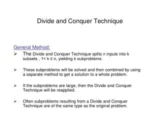
LECTURE 8: Divide and conquer. In the previous lecture we saw …. … how to analyze recursive algorithms write a recurrence relation for the running time solve the recurrence relation by forward or backward substitution … how to solve problems by decrease and conquer

LECTURE 8: Divide and conquer
E N D
Presentation Transcript
LECTURE 8: Divide and conquer Algorithmics - Lecture 8-9
In the previous lecture we saw … … how to analyze recursive algorithms • write a recurrence relation for the running time • solve the recurrence relation by forward or backward substitution … how to solve problems by decrease and conquer • decrease by a constant/variable • decrease by a constant/variable factor … sometimes decrease and conquer lead to more efficient algorithms than brute force techniques Algorithmics - Lecture 8-9
Outline • Basic idea of divide and conquer • Examples • Master theorem • Mergesort • Quicksort Algorithmics - Lecture 8-9
Basic idea of divide and conquer • The problem is divided in several smaller instances of the same problem • The subproblems must be independent (each one will be solved at most once) • They should be of about the same size • These subproblems are solved (by applying the same strategy or directly – if their size is small enough) • If the subproblem size is less than a given value (critical size) it is solved directly, otherwise it is solved recursively • If necessary, the solutions obtained for the subproblems are combined Algorithmics - Lecture 8-9
Basic idea of divide and conquer Divide&conquer (n) IF n<=nc THEN <solve P(n) directly to obtain r> ELSE <Divide P(n) in P(n1), …, P(nk)> FOR i←1,k DO ri← Divide&conquer(ni) ENDFOR r ← Combine (r1, … rk) ENDIF RETURN r Algorithmics - Lecture 8-9
Example 1 Compute the maximum of an array x[1..n] n=8, k=2 3 2 7 5 1 6 4 5 3 2 7 5 1 6 4 5 Divide Conquer 3 2 7 5 1 6 4 5 3 7 6 5 Combine 7 6 7 Algorithmics - Lecture 8-9
Example 1 Efficiency analysis Problem size: n Dominant operation: comparison Recurrence relation: 0, n=1 T(n)= T([n/2])+T(n-[n/2])+1, n>1 Algorithm: Maximum(x[left..right]) IF n=1 then RETURN x[left] ELSE m←(left+right) DIV 2 max1 ← maximum(x[left..m]) max2 ← maximum(x[m+1..right]) if max1>max2 THEN RETURN max1 ELSE RETURN max2 ENDIF ENDIF Algorithmics - Lecture 8-9
Example 1 0, n=1 T(n)= T([n/2])+T(n-[n/2])+1, n>1 Particular case: n=2m 0, n=1 T(n)= 2T(n/2)+1, n>1 Backward substitution: T(2m) = 2T(2m-1)+1 T(2m-1)=2T(2m-2)+1 |* 2 … T(2)=2T(1)+1 |* 2m-1 T(1)=0 ---------------------------- T(n)=1+…+2m-1=2m-1=n-1 Algorithmics - Lecture 8-9
Example 1 0, n=1 T(n)= T([n/2])+T(n-[n/2])+1, n>1 Particular case: n=2m => T(n)=n-1 General case. • Proof by complete mathematical induction First step. n=1 =>T(n)=0=n-1 Inductive step. Let us suppose that T(k)=k-1 for all k<n. Then T(n)=[n/2]-1+n-[n/2]-1+1=n-1 Thus T(n) =n-1 => T(n) belongs to Θ(n). Algorithmics - Lecture 8-9
Example 1 General case. • Smoothness rule If T(n) belongs to (f(n)) for n=bm T(n) is eventually nondecreasing (for n>n0 it is nondecreasing) f(n) is smooth (f(cn) belongs to (f(n)) for any positive constant c) then T(n) belongs to (f(n)) for all n • Remarks. • All functions that do not grow too fast are smooth (polynomial and logarithmic) • For our example (“maximum” algorithm): T(n) is eventually nondecreasing, f(n)=n is smooth, thus T(n) is from (n) Algorithmics - Lecture 8-9
Example 2 – binary search Check if a given value, v, is an element of an increasingly sorted array, x[1..n] (x[i]<=x[i+1]) x1 … xm-1 xm xm+1 … xn v<xm xm=v v>xm x1 … xm’-1 xm’ xm’+1 … xm-1 xm+1 … xm’-1 xm’ xm’+1 … xn True xm=v left>right (empty array) True xleft…..xright False Algorithmics - Lecture 8-9
Example 2 – binary search Remarks: nc=0 k=2 Only one of the two subproblems is solved This is rather a decrease & conquer approach Recursive variant: binsearch(x[left..right],v) IF left>right THEN RETURN False ELSE m←(left+right) DIV 2 IF v=x[m] THEN RETURN True ELSE IF v<x[m] THEN RETURN binsearch(x[left..m-1],v) ELSE RETURN binsearch(x[m+1..right],v) ENDIF ENDIF ENDIF Algorithmics - Lecture 8-9
Example 2 – binary search Second iterative variant: binsearch(x[1..n],v) left ← 1 right ← n WHILE left<right DO m ←(left+right) DIV 2 IF v<=x[m] THEN right ← m ELSE left ← m+1 ENDIF / ENDWHILE IF x[left]=v THEN RETURN True ELSE RETURN False ENDIF First iterative variant: binsearch(x[1..n],v) left ← 1 right ← n WHILE left<=right DO m ←(left+right) DIV 2 IF v=x[m] THEN RETURN True ELSE IF v<x[m] THEN right ← m-1 ELSE left ← m+1 ENDIF / ENDIF/ ENDWHILE RETURN False Algorithmics - Lecture 8-9
Example 2 – binary search • Correctness • Precondition: n>=1 • Postcondition: • “returns True if v is in x[1..n] and False otherwise” • Loop invariant: “if v is in x[1..n] then it is in x[left..right]” • left=1, right=n => the loop invariant is true • It remains true after the execution of the loop body • when right=left it implies the postcondition Second iterative variant: binsearch(x[1..n],v) left ← 1 right ← n WHILE left<right DO m ←(left+right) DIV 2 IF v<=x[m] THEN right ← m ELSE left ← m+1 ENDIF / ENDWHILE IF x[left]=v THEN RETURN True ELSE RETURN False ENDIF Algorithmics - Lecture 8-9
Example 2 – binary search Efficiency: Worst case analysis (n=2m) 1 n=1 T(n)= T(n/2)+1 n>1 T(n)=T(n/2)+1 T(n/2)=T(n/4)+1 … T(2)=T(1)+1 T(1)=1 T(n)=lg n+1 O(lg n) Second iterative variant: binsearch(x[1..n],v) left ← 1 right ← n WHILE left<right DO m ←(left+right) DIV 2 IF v<=x[m] THEN right ← m ELSE left ← m+1 ENDIF / ENDWHILE IF x[left]=v THEN RETURN True ELSE RETURN False ENDIF Algorithmics - Lecture 8-9
Example 2 – binary search Remarks: • By applying the smoothness rule one obtains that this result is true for arbitrary values of n • The first iterative variant and the recursive one also belong to O(lg n) Algorithmics - Lecture 8-9
Master theorem Let us consider the following recurrence relation: T0 n<=nc T(n)= kT(n/m)+TDC(n) n>nc If TDC(n) belongs to (nd) (d>=0) then (nd) if k<md T(n) belongs to (nd lgn) if k=md (nlgk/lgm) if k>md A similar result holds for O and Ω notations Algorithmics - Lecture 8-9
Master theorem Usefulness: • It can be applied in the analysis of divide & conquer algorithms • It avoids solving the recurrencerelation • In most practical applications the running time of the divide and combine steps has a polynomial order of growth • It gives the efficiency class but it does not give the constants involved in the running time Algorithmics - Lecture 8-9
Master theorem Example 1: maximum computation: k=2 (division in two subproblems, both should be solved) m=2 (each subproblem size is almost n/2) d=0 (the divide and combine steps are of constant cost) Since k>md by applying the third case of the master theorem we obtain that T(n) belongs to (nlg k/lg m)= (n) Example 2: binary search k=1 ( only one subproblem should be solved) m=2 (the subproblem size is almost n/2) d=0 (the divide and combine steps are of constant cost) Since k=md by applying the second case of the master theorem we obtain that T(n) belongs to O(nd lg(n))= (lg n) Algorithmics - Lecture 8-9
Efficient sorting • Elementary sorting methods belong to O(n2) • Idea to increase the efficiency of sorting process: • divide the sequence in contiguous subsequences (usually two) • sort each subsequence • combine the sorted subsequences to obtain the sorted sequence Merge sort Quicksort By position Divide By value Combine Merging Concatenation Algorithmics - Lecture 8-9
Merge sort Basic idea: • Divide x[1..n] in two subarrays x[1..[n/2]] and x[[n/2]+1..n] • Sort each subarray • Merge the elements of x[1..[n/2]] and x[[n/2]+1..n] and construct the sorted temporary array t[1..n] . Transfer the content of the temporary array in x[1..n] Remarks: • Critical value: 1 (an array containing one element is already sorted) • The critical value can be larger than 1 (e.g.10) and for the particular case one applies a basic sorting algorithm (e.g. insertion sort) Algorithmics - Lecture 8-9
Merge sort Algorithmics - Lecture 8-9
Mergesort Algorithm: mergesort(x[left..right]) IF left<right THEN m ←(left+right) DIV 2 x[left..m] ← mergesort(x[left..m]) x[m+1..right] ← mergesort(x[m+1..right]) x[left..right] ← merge(x[left..m],x[m+1..right]) ENDIF RETURN x[left..right] Remark: the algorithm will be called as mergesort(x[1..n]) Algorithmics - Lecture 8-9
Mergesort // transfer the last elements of the first array (if it is the case) WHILE i<=m DO k ← k+1 t[k] ← x[i] i ← i+1 ENDWHILE // transfer the last elements of the second array (if it is the case) WHILE j<=right DO k ← k+1 t[k] ← x[j] j ← j+1 ENDWHILE RETURN t[1..k] Merge step: merge (x[left..m],x[m+1..right]) i ← left; j ← m+1; k ← 0; // scan simultaneously the arrays // and transfer the smallest element in t WHILE i<=m AND j<=right DO IF x[i]<=x[j] THEN k ← k+1 t[k] ← x[i] i ← i+1 ELSE k ← k+1 t[k] ← x[j] j ← j+1 ENDIF ENDWHILE Algorithmics - Lecture 8-9
Mergesort • The merge stepcan be used independently of the sorting process • Variant of merge based on sentinels: • Merge two sorted arrays a[1..p] and b[1..q] • Add large values to the end of each array a[p+1]=, b[q+1]= Merge(a[1..p],b[1..q]) a[p+1] ←; b[q+1] ← i ← 1; j ← 1; FOR k ← 1,p+q DO IF a[i]<=b[j] THEN c[k] ← a[i] i ← i+1 ELSE c[k] ← b[j] j ← j+1 ENDIF / ENDFOR RETURN c[1..p+q] Efficiency analysis of merge step Dominant operation: comparison T(p,q)=p+q In mergesort (p=[n/2], q=n-[n/2]): T(n)<=[n/2]+n-[n/2]=n Thus T(n) belongs to O(n) Algorithmics - Lecture 8-9
Mergesort • Efficiency analysis: • 0 n=1 • T(n)= • T([n/2])+T(n-[n/2])+TM(n) n>1 • Since k=2, m=2, d=1 (TM(n) is from O(n)) it follows (by the second case of the Master theorem) that T(n) belongs to O(nlgn). In fact T(n) is from (nlgn) • Remark. • The main disadvantage of merge sort is the fact that it uses an additional memory space of the array size • If in the merge step the comparison is <= then the mergesort is stable Algorithmics - Lecture 8-9
Quicksort • Idea: • Divide the array x[1..n] in two subarrays x[1..q] and x[q+1..n] such that all elements of x[1..q] are smaller than the elements of x[q+1..n] • Sort each subarray • Concatenate the sorted subarrays Algorithmics - Lecture 8-9
Quicksort • An element x[q] having the properties: • x[q]>=x[i], for all i<q • x[q]<=x[i], for all i>q • is called pivot • A pivot is placed on its final position • A good pivot divides the array in two subarrays of almost the same size • Sometimes • The pivot divides the array in an unbalanced manner • Does not exist a pivot => we must create one by swapping some elements Example 1 3 1 2 4 7 5 8 Divide 3 1 2 7 5 8 1 2 3 5 7 8 1 2 3 4 5 7 8 Combine Algorithmics - Lecture 8-9
Quicksort • A position q having the property: • x[i]<=x[i], for all 1<=i<=q and all q+1<=j<=n • is called partitioning position • A good partitioning position divides the array in two subarrays of almost the same size • Sometimes • The partitioning position divides the array in an unbalanced manner • Does not exist such a partitioning position => we must create one by swapping some elements Example 2 3 1 2 7 5 4 8 Divide 3 1 2 7 5 4 8 1 2 3 4 5 7 8 1 2 3 4 5 7 8 Combine Algorithmics - Lecture 8-9
Quicksort The variant which uses a pivot: quicksort1(x[le..ri]) IF le<ri THEN q ← pivot(x[le..ri]) x[le..q-1] ← quicksort1(x[le..q-1]) x[q+1..ri] ← quicksort1(x[q+1..ri]) ENDIF RETURN x[le..ri] The variant which uses a partitioning position: quicksort2(x[le..ri]) IF le<ri THEN q ← partition(x[le..ri]) x[le..q] ← quicksort2(x[le..q]) x[q+1..ri] ← quicksort2(x[q+1..ri]) ENDIF RETURN x[le..ri] Algorithmics - Lecture 8-9
Quicksort • Constructing a pivot: • Choose a value from the array (the first one, the last one or a random one) • Rearrange the elements of the array such that all elements which are smaller than the pivot value are before the elements which are larger than the pivot value • Place the pivot value on its final position (such that all elements on its left are smaller and all elements on its right are larger) • Idea for rearranging the elements: • use two pointers one starting from the first element and the other starting from the last element • Increase/decrease the pointers until an inversion is found • Repair the inversion • Continue the process until the pointers cross each other Algorithmics - Lecture 8-9
Quicksort How to construct a pivot • Choose the pivot value: 4 (the last one) • Place a sentinel on the first position (only for the initial array) • i=0, j=7 • i=2, j=6 • i=3, j=4 • i=4, j=3 (the pointers crossed) • The pivot is placed on its final position 0 1 2 3 4 5 6 7 1 7 5 3 8 2 4 4 1 7 5 3 8 2 4 41 7 5 3 8 24 Pivot value 41 253 874 41 23 5874 41 2 3 4 8 7 5 Algorithmics - Lecture 8-9
Quicksort • Remarks: • x[right] plays the role of a sentinel at the right • At the left margin we can place explicitly a sentinel on x[0] (only for the initial array x[1..n]) • The conditions x[i]>=v, x[j]<=v allow to stop the search when the sentinels are encountered. Also they allow obtaining a balanced splitting when the array contains equal elements. • At the end of the while loop the pointers satisfy either i=j or i=j+1 pivot(x[left..right]) v ← x[right] i ← left-1 j ← right WHILE i<j DO REPEAT i ← i+1 UNTIL x[i]>=v REPEAT j ← j-1 UNTIL x[j]<=v IF i<j THEN x[i]↔x[j] ENDIF ENDWHILE x[i] ↔ x[right] RETURN i Algorithmics - Lecture 8-9
Quicksort Correctness: Loop invariant: If i<j then x[k]<=v for k=left..i x[k]>=v for k=j..right If i>=j then x[k]<=v for k=left..i x[k]>=v for k=j+1..right pivot(x[left..right]) v ← x[right] i ← left-1 j ← right WHILE i<j DO REPEAT i ← i+1 UNTIL x[i]>=v REPEAT j ← j-1 UNTIL x[j]<=v IF i<j THEN x[i]↔x[j] ENDIF ENDWHILE x[i] ↔ x[right] RETURN i Algorithmics - Lecture 8-9
Quicksort Efficiency: Input size: n=right-left+1 Dominant operation: comparison T(n)=n+c, c=0 if i=j and c=1 if i=j+1 Thus T(n) belongs to (n) pivot(x[left..right]) v ← x[right] i ← left-1 j ← right WHILE i<j DO REPEAT i ← i+1 UNTIL x[i]>=v REPEAT j ← j-1 UNTIL x[j]<=v IF i<j THEN x[i]↔x[j] ENDIF ENDWHILE x[i] ↔ x[right] RETURN i Algorithmics - Lecture 8-9
Quicksort Remark: the pivot position does not always divide the array in a balanced manner Balanced manner: • the array is divided in two sequences of size almost n/2 • If each partition is balanced then the algorithm executes few operations (this is the best case) Unbalanced manner: • The array is divided in a subsequence of (n-1) elements the pivot and an empty subsequence • If each partition is unbalanced then the algorithm executes much more operations (this is the worst case) Algorithmics - Lecture 8-9
Quicksort Worst case analysis: 0 if n=1 T(n)= T(n-1)+n+1, if n>1 Backward substitution: T(n)=T(n-1)+(n+1) T(n-1)=T(n-2)+n … T(2)=T(1)+3 T(1)=0 --------------------- T(n)=(n+1)(n+2)/2-3 Thus in the worst case quicksort belongs to (n2) Algorithmics - Lecture 8-9
Quicksort Best case analysis: 0, if n=1 T(n)= 2T(n/2)+n, if n>1 By applying the second case of the master theorem (for k=2,m=2,d=1) one obtains that in the best case quicksort is (nlgn) Thus quicksort belong to Ω(nlgn) and O(n2) An average case analysis should be useful Algorithmics - Lecture 8-9
Quicksort Average case analysis. Hypotheses: • Each partitioning step needs at most (n+1) comparisons • There are n possible positions for the pivot. Let us suppose that each position has the same probability to be selected (Prob(q)=1/n) • If the pivot is on the position q then the number of comparisons satisfies Tq(n)=T(q-1)+T(n-q)+(n+1) Algorithmics - Lecture 8-9
Quicksort The average number of comparisons is Ta(n)=(T1(n)+…+Tn(n))/n =((Ta(0)+Ta(n-1))+(Ta(1)+Ta(n-2))+…+(Ta(n-1)+Ta(0)))/n + (n+1) =2(Ta(0)+Ta(1)+…+Ta(n-1))/n+(n+1) Thus n Ta(n) = 2(Ta(0)+Ta(1)+…+Ta(n-1))+n(n+1) (n-1)Ta(n-1)= 2(Ta(0)+Ta(1)+…+Ta(n-2))+(n-1)n ----------------------------------------------------------------- By computing the difference between the last two equalities: nTa(n)=(n+1)Ta(n-1)+2n Ta(n)=(n+1)/n Ta(n-1)+2 Algorithmics - Lecture 8-9
Quicksort Average case analysis. By backward substitution: Ta(n) = (n+1)/n Ta(n-1)+2 Ta(n-1)= n/(n-1) Ta(n-2)+2 |*(n+1)/n Ta(n-2)= (n-1)/(n-2) Ta(n-3)+2 |*(n+1)/(n-1) … Ta(2) = 3/2 Ta(1)+2 |*(n+1)/3 Ta(1) = 0 |*(n+1)/2 ----------------------------------------------------- Ta(n) = 2+2(n+1)(1/n+1/(n-1)+…+1/3) ≈ 2(n+1)(ln n-ln 3)+2 In the average case the complexity order is n*log(n) Algorithmics - Lecture 8-9
Quicksort -variants 3 7 5 2 1 4 8 v=3, i=1,j=2 3 7 5 2 1 4 8 i=2, j=4 325 7 1 4 8 i=3, j=5 3 2 1 7 5 4 8 i=3, j=8 Plasare pivot: 1 2 3 7 5 4 8 Pivot position: 3 Complexity order of partition: O(n) Another way to construct a pivot pivot(x[left..right]) v←x[left] i ← left FOR j ← left+1,right IF x[j]<=v THEN i ← i+1 x[i] ↔ x[j] ENDIF ENDFOR RETURN i Invariant: x[k]<=v for all left<=k<=i x[k]>v for all i<k<=j Algorithmics - Lecture 8-9
Quicksort -variants 3 7 5 2 1 4 8 v=3 37 5 2 1 4 8 i=2, j=5 31527 4 8 i=3, j=4 3 1257 4 8 i=4, j=3 Partitioning position: 3 Complexity order of partition: O(n) Finding a partitioning position partition(x[left..right]) v ← x[left] i ← left j ← right+1 WHILE i<j DO REPEAT i ← i+1 UNTIL x[i]>=v REPEAT j ← j-1 UNTIL x[j]<=v IF i<j THEN x[i] ↔x[j] ENDIF ENDWHILE RETURN j Remark: The partition algorithm is to be used in the variant quicksort2 Algorithmics - Lecture 8-9
Next lecture will be on … … greedy strategy … and its applications Algorithmics - Lecture 8-9