Weight Learning in Machine Learning: Methods and Optimizations
This overview discusses weight learning in the context of generative and discriminative models, focusing on optimization methods such as gradient descent, Diagonal Newton, and conjugate gradient techniques. The challenges presented by missing data during optimization are addressed, highlighting the use of pseudo-likelihood for improved computation. The effectiveness of various learning rates for different clauses and the implications of ill-conditioning on convergence are analyzed. Key optimization algorithms including Contrastive Divergence and the voted perceptron are examined for their impact on learning efficiency.


Weight Learning in Machine Learning: Methods and Optimizations
E N D
Presentation Transcript
Weight Learning Daniel Lowd University of Washington <lowd@cs.washington.edu>
Overview • Generative • Discriminative • Gradient descent • Diagonal Newton • Conjugate Gradient • Missing Data • Empirical Comparison
Weight Learning Overview Weight learning is function optimization. • Generative learning: • Discriminative learning: • Learning with missing data: Typically too hard! Use pseudo-likelihood instead Used in structure learning Most common scenario. Main focus of class today. Modification of discriminative case.
Optimization Methods • First-order Methods • Approximate f(x) as a plane: • Gradient descent (+ various tweaks) • Second-order Methods • Approximate f(x) as quadratic form: • Conjugate gradient – “correct” the gradient to avoid undoing work • Newton’s method – use second derivatives to move directly towards optimum • Quasi-Newton methods – approximate Newton’s method using successive gradients to estimate curvature
f(w) w w2 w1 Convexity (and Concavity) Formally: 1D: 2D:
Generative Learning • Function to optimize: • Gradient: Counts in training data Weighted sum over all possible worlds No evidence, just sets of constants Very hard to approximate
Pseudo-likelihood • Efficiency tricks: • Compute each nj(x) only once • Skip formulas in which xl does not appear • Skip groundings of clauses with > 1 true literale.g., (A v ¬B v C) when A=1, B=0 • Optimizing pseudo-likelihood • Pseudo-log likelihood is convex • Standard convex optimization algorithms work great (e.g., L-BFGS quasi-Newton method)
Pseudo-likelihood • Pros • Efficient to compute • Consistent estimator • Cons • Works poorly with long-range dependencies
Discriminative Learning • Function to optimize: • Gradient: Counts in training data Weighted sum over possibleworlds consistent with x.
Approximating E[n(x,y)] • Use the counts of the most likely (MAP) state • Approximate with MaxWalkSAT -- very efficient • Does not represent multi-modal distributions well • Average over states sampled with MCMC • MC-SAT produces weakly correlated samples • Just a few samples (5) often suffices! (Contrastive divergence) • Note that a single complete state may have millions of groundings of a clause! Tied weights allow us to get away with fewer samples.
Approximating Zx • This is much harder to approximate than the gradient! • So instead of computing it, we avoid it • No function evaluations • No line search • What’s left?
Gradient Descent Move in direction of steepest descent, scaled by learning rate: wt+1 = wt + gt
Gradient Descent in MLNs • Voted perceptron [Collins, 2002; Singla & Domingos, 2005] • Approximate counts use MAP state • MAP state approximated using MaxWalkSAT • Average weights across all learning steps for additional smoothing • Contrastive divergence [Hinton, 2002; Lowd & Domingos, 2007] • Approximate counts from a few MCMC samples • MC-SAT gives less correlated samples [Poon & Domingos, 2006]
Per-weight learning rates • Some clauses have vastly more groundings than others • Smokes(x) Cancer(x) • Friends(a,b) Friends(b,c) Friends(a,c) • Need different learning rate in each dimension • Impractical to tune rate to each weight by hand • Learning rate in each dimension is: /(# of true clause groundings)
Problem: Ill-Conditioning • Skewed surface slow convergence • Condition number: (λmax/λmin) of Hessian
The Hessian Matrix • Hessian matrix: all second-derivatives • In an MLN, the Hessian is the negative covariance matrix of clause counts • Diagonal entries are clause variances • Off-diagonal entries show correlations • Shows local curvature of the error function
Newton’s Method • Weight update: w = w + H-1 g • We can converge in one step if error surface is quadratic • Requires inverting the Hessian matrix
Diagonalized Newton’s method • Weight update: w = w +D-1g • We can converge in one step if error surface is quadratic AND the features are uncorrelated • (May need to determine step length…)
Problem: Ill-Conditioning • Skewed surface slow convergence • Condition number: (λmax/λmin) of Hessian
Conjugate Gradient • Gradient along all previous directions remains zero • Avoids “undoing” any work • If quadratic, finds n optimal weights in n steps • Depends heavily on line searchesFinds optimum along search direction by function evals.
Scaled Conjugate Gradient [Møller, 1993] • Gradient along all previous directions remains zero • Avoids “undoing” any work • If quadratic, finds n optimal weights in n steps • Uses Hessian matrix in place of line search • Still cannot store full Hessian in memory
Choosing a Step Size [Møller, 1993; Nocedal & Wright, 2007] • Given a direction d, how do we choose a good step size α? • Want to make gradient zero. Suppose f is quadratic: • But f isn’t quadratic! • In a small enough region it’s approximately quadratic • One approach: Set maximum step size • Alternately, add a normalization term to denominator
How Do We Pick Lambda? • We don’t. We adjust it automatically. • According to the quadratic approximation, • Compare to the actual difference, • If ratio is near one, decrease λ • If ratio is far from one, increase λ • If ratio is negative, backtrack! • We can’t actually compute , but we can exploit convexity to bound it.
How Convexity Helps f(w) wt-1 wt wt – wt-1
How Convexity Helps Slope Step t f(w) wt-1 wt wt-1 - wt
How Convexity Helps Slope Step t f(w) wt-1 wt wt-1 - wt
Step Sizes and Trust Regions • By using the lower bound in place of the actual function difference, we ensure that f(x) never decreases. • We don’t need the full Hessian, just dot products Hv. We can compute this directly from samples: • Other tricks • When backtracking, take new samples at the old weight vector and add them to the old samples • When the upper bound on improvement falls below a threshold, stop. [Perlmutter, 1994]
Preconditioning • Initial direction of SCG is the gradient • Very bad for ill-conditioned problems • Well-known fix: preconditioning • Multiply by matrix to lower condition number • Ideally, approximate inverse Hessian • Standard preconditioner: D-1 [Sha & Pereira, 2003]
Overview of Discriminative Learning Methods • Gradient descent • Direction: Steepest descent • Step size: Simple ratio • Diagonal Newton • Direction: Shortest path towards global optimum, assuming f(x) is quadratic and clauses are uncorrelated • Step size: Trust region • Much more effective than gradient descent • Scaled conjugate gradient • Direction: Correction of gradient to avoid “undoing” work • Step size: Trust region • A little better than gradient descent without preconditioner;a little better than diagonal Newton with preconditioner
Learning with Missing Data Gradient: We can use inference to compute each expectation. However, the objective function is no longer convex. Therefore, extra caution is required when applying PSCG or DN – you may need to adjust λ more conservatively.
Practical Tips There are several reasons why discriminative weight learning can fail miserably… • Overfitting • How to detect: Evaluate model on training data • How to fix: Use narrower prior (-priorStdDev) or change the set of formulas • Inference variance • How to detect: Lambda grows really large • How to fix: Increase MC-SAT samples (-minSteps) • Inference bias • How to detect: Evaluate model on training data.Clause counts should be similar to during training. • How to fix: Re-initialize MC-SAT periodically during learning or change set of formulas.
Experiments: Algorithms • Voted perceptron (VP,VP-PW) • Contrastive divergence (CD,CD-PW) • Diagonal Newton (DN) • Scaled conjugate gradient (SCG, PSCG)
Experiments: Cora [Singla & Domingos, 2006] • Task: Deduplicate 1295 citations to 132 papers • MLN (approximate): HasToken(+t,+f,r) ^ HasToken(+t,+f,r’) => SameField(f,r,r’) SameField(+f,r,r’) <=> SameRecord(r,r’) SameRecord(r,r’) ^ SameRecord(r’,r”) => SameRecord(r,r”) SameField(f,r,r’) ^ SameField(f,r’,r”) => SameField(f,r,r”) • Weights: 6141 • Ground clauses: > 3 million • Condition number: > 600,000
Experiments: WebKB [Craven & Slattery, 2001] • Task: Predict categories of 4165 web pages • MLN: PageClass(page,class) HasWord(page,word) Links(page,page) HasWord(p,+w) => PageClass(p,+c) !HasWord(p,+w) => PageClass(p,+c) PageClass(p,+c) ^ Links(p,p') => PageClass(p',+c') • Weights: 10,891 • Ground clauses: > 300,000 • Condition number: ~7000