Download

1 / 25
270 likes | 672 Views
DUMMY VARIABLES. BY HARUNA ISSAHAKU. Definition. Dummy variables (DV) indicate the presence or absence of a ‘quality’ or an attribute such as male or female, black or white, north or south, etc.

E N D
DUMMY VARIABLES BY HARUNA ISSAHAKU Haruna Issahaku
Definition • Dummy variables (DV) indicate the presence or absence of a ‘quality’ or an attribute such as male or female, black or white, north or south, etc. • A dummy variable will take the value 1 or 0 according to whether or not the condition is present or absent for a particular observation. Haruna Issahaku
1 indicates the presence of the attribute • 0 indicates the absence of the attribute • Eg. 1 may represent female and 0 for male • DV are sometimes called categorical variables, or qualitative variables or indicator variables • ANOVA MODELS: Used to test the statistical significance of the relationship between a quantitative regressand and qualitative or dummy regressors Haruna Issahaku
ANCOVA MODELS: regression models containing an admixture of quantitative and dummy regressors. • They provide a method of statistically controlling for the effects of quantitative regressors called covariates or control variables in a model that includes both quantitative and qualitative regressors Haruna Issahaku
A single dummy independent variable • Given the wage discrimination model • Wage=hourly wage • D=1 for females and 0 for males • is the difference in hourly wage between males and females given the same level of education and the same error term u. • is the mean hourly wage for males (the base or benchmark group) Haruna Issahaku
Why a single category is included in a single DV. equation • Using two DV would introduce perfect colinearity because for example • Female + male=1 • Ie. Male is a perfect colinear function of female • Introducing DV for both male and female is the simplest example of the so called dummy variable trap. • It arises when too many DV describe a given number of groups Haruna Issahaku
Overcoming the DV trap • One way of overcoming the DV trap is to drop the intercept and include the two categories • Eg. Haruna Issahaku
Some interpretations • Given • Wage = 2.91 - 1.81female + 0.572educ. • Se= (0.12) (0.26) (0.049) • N=526 R-sqd=0.364 • -males receive a mean wage of Ghc2.91 per hour • -on the average females receive Ghc1.81 less than their male counterparts holding education constant. • -the average hourly wage of female is • 2.91-1.81=Ghc1.10 Haruna Issahaku
Interpreting coefficients on DV when an explanatory v. is in log form • Given the ff. model on the effects of training grants on hours of training by firms • hrsemp=hours of training per employee at the firm level • Grant is a DV =1 if a firm received a job training grant and 0 otherwise Haruna Issahaku
Sales=annual sales • Employ=total no. of employees of the firm • Grant coefficient of 26.25 means controlling for sales and employment, firms that receive grants trained each worker on the average 26.25 hours more • The coefficient on log sales is small and insignificant Haruna Issahaku
The coefficient on log employ of -6.07 means • If a firm is 1% larger it trains its workers by 0.061 (ie. 6.07/100) hours less Haruna Issahaku
Interpreting DV when dependent v. is in log form • 1. given the housing price equation • Colonial is a DV. =1 if house is of a colonial style and 0 otherwise • Raw interpretation: holding other factors constant the difference in log(price) of a house of a colonial style is 0.054 • Correct interpretation: a house of the colonial style is predicted to sell for about 5.4% more, holding other factors constant • Ie. When the dependent v. is in log form the coefficient on the DV multiplied by 100 is interpreted as percentage difference in the dependent variable holding other factors constant. Haruna Issahaku
2. Given a log hourly wage equation • Using log(wage) as the dependent v. and adding quadratics in experience • The coefficient on female implies for the same levels of experience and education women on the average earn 29.7% (ie. 100*0.297) less than men • More accurate interpretation: a more accurate interpretation is obtained by using the formula Haruna Issahaku
100*[exp.(B)-1] • Where B is the coefficient on the dummy variable • Thus, 100*[exp.(-0.297)-1]=25.7 • More accurately, on the average a woman’s wage is 25.7% below a comparable man’s wage Haruna Issahaku
Median hourly wage for males is calculated by taking the antilog of the intercept 0.417 • exp(0.417)=Ghc1.517 • The median hourly wage of females • Exp[0.417+(-0.279)]=Ghc1.148 Haruna Issahaku
ANOVA models with 2 DV. • Model: hourly wage in relation to marital status and region of residence • Y=hourly wage (Ghc) • =marital status 1=married 0=otherwise • =region of residence 1=south 0=otherwise Haruna Issahaku
Which is the benchmark group? • Unmarried non-south residents • All comparisms are made wrt this group as ff: • -Unmarried non-south residents receive a mean hourly wage of GhC8.81 • -Those married on average receive Ghc1.10 more than the unmarried non-south residents Haruna Issahaku
The mean hourly wage for the married is Ghc 9.91 (ie. 8.81+1.10) • -the hourly wage of those from the south is lower by Ghc 1.67 • The mean hourly wage of those from the south is Ghc7.14 (ie. -1.67+8.81) • All are statistically significant. Haruna Issahaku
Interaction effects using DV. • Given • Female is a dummy=1 for females; 0=otherwise • Married is a dummy 1=married 0=otherwise • The differential effect of being a married female is 0.301 • Married females earn 35.12% more than single men with a mode of Ghc1.35 Haruna Issahaku
What will be the earnings for • 1. married men? • 2. single men? • 3. unmarried females? Haruna Issahaku
Uses of DV in applied econometric research • Read Akoutsoyannis pp.281-284 • 1. As proxies to qualitative variables • 2. As proxies for numerical factors • 3. Measuring shifts of a function over time • 4. Measuring the change in parameters over time • 5. As proxies for the dependent variable • 6. For seasonal adjustment of time series Haruna Issahaku
Indicator vs effects coding • Indicator coding: where the reference category is assigned zero across the set of DV. • Effects coding: where the reference category is assigned a value of negative 1 across the set of DV. • In indicator coding coefficients represent group deviations on the dependent variable from the reference group • While in effect coding coefficients become group deviations on the dependent variable from the mean of the dependent variable across all groups Haruna Issahaku