Download

1 / 22
220 likes | 255 Views
Modeling of Traffic Flow Problems. Prof. S. Sundar. Plan. Introduction Traffic Flow Models Traffic Flow for single lane (Lighthill-Whitham) Traffic Flow for single lane with traffic jam Traffic Flow for two lane with traffic jam Numerical Approximations to Linear Scalar Conservation Laws

E N D
Modeling of Traffic Flow Problems Prof. S. Sundar
Plan • Introduction • Traffic Flow Models • Traffic Flow for single lane (Lighthill-Whitham) • Traffic Flow for single lane with traffic jam • Traffic Flow for two lane with traffic jam • Numerical Approximations to Linear Scalar Conservation Laws • Central Difference Scheme • Lax-Friedrich’s Scheme • Down-Wind Scheme • Up-Wind Scheme • Numerical Approximations to Non-Linear Scalar Conservation Laws
Introduction x1 xx2 The number of cars in the interval (x1,x2) Traffic Flow Cars High Way The density of cars (number of cars per km.) The number of cars which pass through x at time t The number of cars in the interval (x1,x2) changes according to the number of cars which enter or leave this interval. On Simplification Conservation Law
Scalar Conservation Law And can be solved using the method of characteristics The solutions may develop discontinuties after a finite time Weak Solution Riemann Problem
Lighthill-Whitham model for a single lane Scalar Conservation Law – Equation of motion With non-linear flux function 0< < max Where umax is the maximum attainable velocity of cars in traffic If the highway is empty ( = 0), we drive with maximal velocity And in heavy traffic, we tend to slow down, and in a tailback the carks are bumper to bumper (= max )
Propagation on a single lane with a traffic jam The Lighthill-Whitham model for a single lane In a traffic jam situation, the flow of traffic at one place is limited and the flow at some other part of the road is different. Which means, we have different density function at different parts of the road.
Propagation on two lanes with a traffic jam We use the similar model but with a source term on the right to depict the merging of lines 1 Main Road The source term would include the rate of change of cars within the region x1-x0, beyond which we assume that there are no other merging roads x1 x0 2 Merging Road Is the rate at which the cars change from one lane to another, 0, 1 are initial densities.
(i,n+1) (i-1,n+1) (i+1,n+1) t (i-1,n) (i+1,n) (i,n) (i,n-1) (i+1,n-1) (i-1,n-1) x For example Taylor series expansion of the above equation Numerical Approximation of Linear Scalar Conservation Laws A simple linear scalar conservation law where Now, we discretize the (x,t) plane For simplicity we take a uniform mesh with h and k constant The simplest of approximations to the solution at these grid points is the finite difference approximation i.e., to replace partial derivatives by difference quotients.
(i,n+1) (i-1,n+1) (i+1,n+1) t (i-1,n) (i+1,n) (i,n) (i,n-1) (i+1,n-1) (i-1,n-1) x Equivalently, This is an implicit scheme, where a linear system has to be solved Central Difference Scheme A simple linear scalar conservation law Using the Central Difference Approximation (in space only ??) Which can be re-written as As we can compute uin+1 from the data uin explicitly, this is known as explicit scheme
Boundary Conditions In Practice, we compute on a finite grid say x in (0,a) and we require appropriate Boundary Conditions. Periodic Boundary Conditions Discretized version Setting i=0 or i=N, we required to determine u-1n or uN+1nand we consider these points as artificial points with By periodicity
Numerical Implementation Discontinuous Initial Data Continuous Initial Data h = 0.01 k = 0.001 x = 0 to 1 t = 0 to 0.25
u x
(i,n+1) (i-1,n+1) (i+1,n+1) t (i-1,n) (i+1,n) (i,n) (i,n-1) (i+1,n-1) (i-1,n-1) x Lax-Friedrich’s Scheme The time derivative is approximated using And the spatial derivative is approximated using the central difference scheme Hence, the scheme is We will see that the solution is smeared out, and this approximation becomes better and better for smaller k>0
Numerical Implementation Discontinuous Initial Data Continuous Initial Data h = 0.01 k = 0.001 x = 0 to 1 t = 0 to 0.25
(i,n+1) (i-1,n+1) (i+1,n+1) t (i-1,n) (i+1,n) (i,n) We will see that the numerical solution is unstable (i,n-1) (i+1,n-1) (i-1,n-1) The solution describes a wave from left to right. x Down-Wind Scheme The Lax-Friedrich’s scheme gives accurate approximations only if k is sufficiently small. The Down-Wind scheme is described by
Numerical Implementation Discontinuous Initial Data Continuous Initial Data h = 0.01 k = 0.001 x = 0 to 1 t = 0 to 0.25
(i,n+1) (i-1,n+1) (i+1,n+1) t (i-1,n) (i+1,n) (i,n) (i,n-1) (i+1,n-1) (i-1,n-1) x Up-Wind Scheme In the Down-Wind Scheme, the spatial derivative at xi uses the information at xi+1 where the wave will go in the next time step, which does not make sense. It would be more reasonable to use the information at xi-1 where the wave comes from. Hence, the Up-wind Scheme is described as We will see that, the solution is almost exact
Numerical Implementation Discontinuous Initial Data Continuous Initial Data h = 0.01 k = 0.001 x = 0 to 1 t = 0 to 0.25
Numerical Approximation of Non-Linear Scalar Conservation Laws Up-Wind Scheme Lax-Friedrich’s Scheme Quasi-Linear equation Conservation form