Fundamental Principles of Traffic Flow

1. Fundamental Principles of Traffic Flow Chapter 6 Dr. TALEB AL-ROUSAN

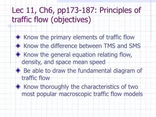
2. Introduction • Traffic flow theory involves the development of mathematical relationships among the primary elements of a traffic stream> • Flow • Density • Speed • These relationships help traffic engineer in planning, designing, and evaluating the effectiveness of implementing traffic engineering measures on a highway system.

3. Applications of Traffic Flow Theory • Traffic flow theory is used in design to determine: • Adequate lane length for storing left-turn vehicles on separate left-turn lanes. • Average delay at intersections and freeway ramp merging areas. • Changes in the level of freeway performance due to the installation of improved vehicular control devices on ramps. • Traffic flow theory is used in simulation: • Mathematical algorithms are used to study the complex interrelationship between elements of traffic stream. • Estimate the effect of changes in traffic flow on factors such as accidents, travel time, air pollution, and gasoline consumption.

4. Traffic Flow Elements • Time-space diagram: A graph the describes the relationship between the location of vehicles in a traffic stream and the time as the vehicles progress along the highway. • See Figure 6.1. • (X,Y) = (Time, Distance) • Primary elements are: flow, density, & speed. • Another element, associated with density, is the gap or headway between vehicles in traffic stream

6. Traffic Flow Elements Definitions • Flow (q) : the equivalent hourly rate at which vehicles pass a point on a highway during a time period less than 1 hour. q= [(n x 3600)/T]……veh/h n = number of vehicles passing a point in the roadway in (T) seconds. • Density (k) : ,also referred to as concentration, number of vehicles traveling over a unit length (usually one mile) of highway at an instant in time. Unit of density is (vehicle/mi)

7. Traffic Flow Elements Definitions Cont. • Speed (u) : the distance traveled by a vehicle during a unit of time (mi/h) or (km/h) or (ft/sec), • The speed of a vehicle at any time (t) is the slope of the time-space diagram for that vehicle at time (t). • Two types of mean speed: • Time mean speed • Space mean speed

8. Traffic Flow Elements Definitions Cont. • Time Mean Speed (ūt) :the arithmetic mean of the speeds of vehicles passing a point on a highway. ūt = [(1/n) (Sum (ui)) ]…. i = 1 to n n= number of vehicles passing a point on a highway. ui = speed of the ith vehicle (ft/sec)

9. Traffic Flow Elements Definitions • Space Mean Speed (ūs) :the harmonic mean of the speeds of vehicles passing a point on a highway during an interval of time. • Obtained by dividing the total distance traveled by two or more vehicles on a section of a highway by the total time required by these vehicles to travel that distance. • Space mean speed is the one involved in flow-density relationship. ūs = [n/ (Sum (1/ui)) ]…. i = 1 to n ūs = [nL / (Sum (ti)) ]…. i = 1 to n n= number of vehicles passing a point on a highway. ui = speed of the ith vehicle (ft/sec). ti = the time it takes the ith vehicle to travel a cross a section of highway (sec). L= length of section of highway (ft).

10. Traffic Flow Elements Definitions Cont. • The time mean speed is always higher than the space mean speed. • The difference between these speeds tends to decrease as the absolute values of speeds increase. ūt = ūs + (s2/ ūs)

11. Traffic Flow Elements Definitions Cont. • Time Headway (h): is the difference between the time the front of a vehicle arrives at a point on the highway and the time the front of the next vehicle arrives at that same point, expressed in (seconds).. • Can be found from time-space diagram at specified distance. • Space Headway (d): is the distance between the front of a vehicle and the front of the following vehicle, expressed in (feet). • Can be found from time-space diagram at specified time (t). • See Example 6.1

12. Flow-Density Relationships • The general equation relating flow, density, and space mean speed is given as: • Flow = density x space mean speed q= k ūs • Each of variable depends on several other factors, including: • Characteristics of the roadway. • Characteristics of the vehicle • Characteristics of the driver • Environmental factors (e.g. weather)

13. Flow-Density Relationships Cont. • Other relationships exist among traffic flow variables> • Space mean speed = (flow) x (average space headway) ūs = q đ average space headway = đ = (1/k) • Density = (flow) x (average travel time for unit distance) K= q Ť • Average space headway = (space mean speed) x (average time headway) đ = ūs Ћ • Average time headway = (average travel time for unit distance) x (average space headway) Ћ = Ť đ

14. Fundamental Diagram of Traffic Flow • See Figure 6.4 • Flow vs. Density: • When there are no vehicles on the highway, the density is zero and flow is also zero. • As density increase flow also increase. • When density reaches max. (jam density Kj), the flow must be zero because vehicles will tend to line up end to end. • It follows that as density increases from zero, the flow will also initially increase from zero to a max. value. • Further continuous increase in density will then result in continuous reduction of flow, which will be zero when density is equal to the jam density. • See Figure 6.4a • Some controversy exist regarding the exact shape of the curve.

16. Fundamental Diagram of Traffic Flow Cont. • Space Mean Speed vs. Flow: • When flow is very low, there is little interaction between vehicles, therefore drivers are free to travel at max possible speed. • The absolute max speed is obtained as the flow tends to zero (Mean Free Speed uf ). • Magnitude of (uf) depends on the physical characteristics of the highway. • Continuous increase in flow will result in a continuous decrease in speed. • A point will be reached when further addition of vehicles will result in the reduction in the actual number of vehicles that pass a point on the highway (reduction of flow). • At this point congestion is reached and eventually both speed and flow become zero. • See Figure 6.4 c.

18. Fundamental Diagram of Traffic Flow Cont. • Space Mean Speed vs. Density: • When there are no vehicles on the highway, the density is zero. • When density is zero there will be little or no interaction between vehicles, therefore drivers are free to travel at max possible speed. • Further continuous increase in density will then result in continuous reduction of speed, which will be zero when density is equal to the jam density • See Figure 6.4 b.

19. Fundamental Diagram of Traffic Flow Cont. • knowing that: [ūs = q/k ] means that slopes of lines (OB, OC, OE) in Figure 6.4a represent the space mean speeds at densities (Kb, kc, ke) respectively. • Slope of OA = the speed at density tends to zero = mean free speed (uf) = max speed that can be attained on the highway. • Slope of OE = the speed for max flow = capacity of the highway. • It is desirable for highways to operate at densities not greater than that required for maximum flow.

20. Mathematical Relationships Describing Traffic Flow • Macroscopic approach: considers flow-density relationship. 1- Greenshields Model: used for light or dense traffic (satisfies boundary conditions when density approach zero or jam density). ūs = uf– ((uf /kj)k) q = (uf k )– ((uf /kj) k2) 2- Greenberg model: used only for dense traffic (satisfies boundary conditions when density approach jam density). ūs = c ln (kj/k) q = ūs k = c k ln (kj/k) • Microscopic approach: (referred to as car-following theory or follow-the-leader theory) considers spacing between vehicles and speeds of individual vehicles.

21. Gap & Gap Acceptance • Another important aspect of traffic flow is the interaction of vehicles as they: • Join a traffic stream : ramp vehicles merging into an expressway stream. • Leave a traffic stream : freeway vehicles leaving the freeway onto frontage roads. • Cross a traffic stream: changing of lanes by vehicles on a multilane highway. • the most important factor a driver consider in making any of these maneuvers is the availability of a gap between two vehicles that, in drivers judgment, is adequate for him/her to complete the maneuver.

22. Important Measures In Concept of Gap Acceptance • Merging: the process by which a vehicle in one traffic stream joins another traffic stream in the same direction. • Diverging: the process by which a vehicle in a traffic stream leaves the traffic stream. • Weaving: the process by which a vehicle first merges into a stream of traffic obliquely crosses that stream, and them merges into a second stream moving in the same direction.

23. Important Measures In Concept of Gap Acceptance • Gap: the headway in a major stream, which is evaluated by a vehicle driver in the minor stream who wishes to merge into the major stream. Expressed in units of (time or distance) • Time Lag: the difference between the time a vehicle that merges into a main traffic stream reaches a point on the highway in the area of merge and the time a vehicle in the main stream reaches the same point. • Space lag: the difference, at an instant of time, between the distance a merging vehicle is a way from a reference point in the area of merge and the distance a vehicle in the main stream is a way from the same point.

24. Gap Acceptance