Multi-view shape reconstruction
Multi-view shape reconstruction. Shape reconstruction. Approach: chose a surface representation define a photo-consistency function [in practice photo-consistency+regularization] solve the following minimization. Given A set of images (views) of an object / scene

Multi-view shape reconstruction
E N D
Presentation Transcript
Shape reconstruction Approach: • chose a surface representation • definea photo-consistency function [in practice photo-consistency+regularization] • solve the following minimization Given • A set of images (views) of an object / scene • Camera calibration information • [Light calibration information] Find the surface that best agrees with the input images. …
Photo-consistency function(al) Extension SFS/PS to multi-view: Needs camera/light calibration ! Move camera Move object PS SFS Based on image cues (shading, stereo, silhouettes, …)
Surface representation Image-centered Object-centered • Depth/disparity w.r. to image plane • Voxels • Level sets (implicit) • Mesh • Depth with respect to a base mesh • Local patches time 3D point Image plane 3D plane Partial object reconstr. Limited resolution Viewpoint dependent
Comparison of different methods 2 datasets No light (moving camera)
Volumetric representation Object : collection of voxels Normals : ? Method: carve away voxels that are not photo-consistent with images (purely discrete) Regularization: no way of ensuring smoothness Visibility: ensured by the order of traversal (in general a problem!)
Disparity/Depth map 3D point Reference image Reference image plane Object (surface) : Normals : Method: find f that best agrees with the input images (minimize the cost functional integrated over the surface) Regularization: smoothness on Visibility: ? (mesh defined on image plane + Zbuffering)
Depth w.r. base mesh Object (surface) : , d – displacement direction (displacement map) Normals : local (per triangle) transform to global CS Method: Regularization: smoothness on (local / global) Visibility: ? (fine mesh to connect points on each plane + Zbuffering) How to deal with boundaries ?
Mesh Object (surface) : mesh vertices Normals :interpolated Method: move vertices along interpolated normals based on photo-consistency of neighboring triangles. Regularization: smooth normals Visibility: Zbuffering Topologiocal changes ?
Mixed Representations:Local patches • Mixed approaches : • patches on voxels for a finer surface representation • mesh on pre-computed voxel correlation (potential fields) [Esteban and Schmitt CVIU 2005] • (depth on base mesh) Patches : • arbitrary : [Zheng, Paris et al. IJCV2006] • quadratic : surfels [Carceroni and Kutulakos IJCV 2002]
Optimization Graph-cuts Belief propagation Dynamic programming… Discrete methods Non-linear optimization Variational calculus Continuous methods Voxel carving (exhaustive search For same color) Disparity map Depth w.r.plane Level sets Mesh Voxels
Summary Discrete • Voxel carving • Graph cut techniques Continuous • Variational and level set techniques • Mesh-based reconstruction
Shape from Silhouette Binary images • Back project each silhouette 3D cone. • Carve all voxels outside the cone. • Result: • Reconstruction contains the true scene, but not the same (no concavities) • Not photo-consistent (only to binary images). • In the limit reconstructs a visual hull [Martin PAMI 91][Szeliski 93] + Our capgui in lab
Smarter volumetric representations Voxel-based Image ray based Axis-aligned + Moderatly accurate + Fast + Marching intersections Tarini’01 + our Capgui • Inaccurate • + Triangulate w. marching cubes + Accurate Franco, Boyer
Volumetric reconstruction Method : Carve voxels that are not consistent with images (according to a chosen photo-consistency score). OR Assign colors to voxels consistent with the input images. (color + opacity) Not unique solution True scene N3 voxels C colors Order of traversal v. important all scenes Photo-consist. scenes
Voxel coloring • Each voxel • Project in images and correlate • Color if consistent Visibility ! Depth ordering : Single visibility ordering for each view (Restriction in camera placement) [Seitz,Dyer CVPR97] Plane sweep [Collins CVPR 96] No scene point contained within the convex hull of the cameras Traversal order
Voxel coloring : results Input image Results [Seitz,Dyer CVPR97]
Space carving In general a view independent order might not exist • Space carving[Kutulakos, Seitz ICCV 99, IJCV 2002] • initialize a volume containing the scene • Choose a voxel on the surface of the scene • Project in all visible images • Carve if not consistent • Repeat until convergence Consistency: The resulting shape is photo-consistent (all inconsistent voxels are removed) Convergence: Carving converges to a non-empty shape (a point on the true surface is never removed) Photo-hull
Space carving : photo hull Initial volume and true scene Photo-hull • Photo-hull = union of all photo-consistent shapes • Basic algorithm : requires a difficult update procedure (visibility computation after carving a voxel) • Multi-pass plane sweep : • Sweep plane in each 6 directions • Consider active only cameras on one side of the plane
Space carving : results [Kutulakos, Seitz ICCV 99, IJCV 2002]
Graph cuts for multi-view reconstruction • Discrete surface reconstruction • Graph cut • Graph cuts as hypersurfaces • Example: [Paris, Sillion, Quan IJCV 05] • Types of energies minimized with graph cut [Kolmogorov Zabih ECCV 2002] • Graph cuts for multi-labeling
Reconstruction as labeling Photo-consistency Smoothness Ex: disparity mapvoxels pixels voxels disparities occupancy Discrete formulation: • surface representation • labels Find a set of labels that minimize Notes: • NP hard • Can be solved using MRF energy minimization methods graph cuts (submodular E), dynamic programming, belief propagation, simulated annealing …
Graph cuts • Oriented graph • nodes • edges V , source s , sink t E , edge capacity w(p,q) (non-negative) Cut C={S,T} partition of nodes into two disjoint sets such that sS, t T Cost of the cut Minimum cut cut that has minimum cost among all cuts (binary labeling) Maximum flow maximum amount of liquid that can be sent from the source to the sink interpreting edges as pipes with capacity w. Polynomial time algorithms Augmenting paths [Ford & Fulkerson, 1962] Push-relabel [Goldberg-Tarjan, 1986]
Energy minimization via graph cuts • Motivation: • Geometric interpretation cut = hypersurface in N-D space embedding the corresponding graph used to compute optimal hypersurface • Powerful energy minimization tool for a large class of binary and non-binary energies global minimum; strong local minimum • Surface reconstruction: • Chose a surface representation • Define a graph (nodes, weights) such that the cost of a cut corresponds to the surface energy function. How to find global labeling using graph cut ? What kind of energy can be minimized with a graph cut ?
Graph Cuts as Hypersurfaces labels t “cut” y s p x cut • Graph fully embedded in the working geometric space • Feasible cut = separated hypersurface in the embedding continuous manifold
Comparison to “stereo” labels “cut” labels L(p) L(p) y p x x p Multi-scanline optimization s-t Graph Cuts multi-scan-line optimization single scan line optimization eg Search, Dynamic Programming 26
Example of geometric graph [Paris, Sillion, Quan: A surface reconstruction method using global graph cut optimization IJCV 05] Disparity map: pixel label = disparity source D4(d1) D1(d1) ’ ’ ’ d1 D1(d2) D2(d2) D4(d2) D3(d2) d2 f1=d4 f2=d3 f3=d3 f4=d4 D4(d3) d3 D4(d4) ’ ’ ’ d4 sink Surface Graph
Results Convex smoothing – global solution [Paris, Sillion, Quan IJCV 05, ACCV 04]
Types of regularization energies • Convex • + global convergence • oversmooth V(Δf) linear Δf=fp-fq Preserves discontinuities NP hard ? convergence V(Δf) Δf=fp-fq Potts piecewise planar binary graph V(Δf) Potts Δf=fp-fq
Exact multi-labeling t s Linear and convex smoothing (interaction) energy Geometric graphs. • Multi-scan-line stereo [Roy & Cox 1998, 1999] [Ishikawa & Geiger 1999] (occlusion handling) • “Linear” interaction energy [Ishikawa & Geiger 1998] [Boykov, Veksler, Zabih 1998] • Convex interaction energy • [Ishikawa 2000, 2003]
Binary graphs a cut n-links t-link t t-link s [Kolmogorov, Zabih : What energy functions can be minimized via graph cuts? ECCV 2002] Complete characterization of energies that can be minimized with graph cut : E(f) can be minimized by s-t graph cuts Large class of energies (Potts, metric …) BUT multi-view reconstruction is a multi-labeling problem !
Approximate multi-labeling cut n-links [ Boykov et al: Fast approximate energy via graph cuts, PAMI 2001] t-link • Expansion approximate solution • Ideea: break optimization into a set of binary s-t cut problems • Each iteration – consider one label a • Binary cut: some labels are relabeled with a; the others remain unchanged t a t-link current label s Binary Potts energy Extended to multi-labeling NP hard ( 3 labels)
- expansion Examples of standard and large moves from a given iniotia; labeling. The number of labels is |L| = 3. initial labeling standard move swap a-expansion
expansion simulated annealing, 19 hours, 20.3% err normalized correlation, start for annealing, 24.7% err a-expansions (BVZ 89,01) 90 seconds, 5.8% err • Properties Guaranteed approximation quality • within a factor of 2 from the global minima (Potts model) Applies to a wide class of energies with robust interactions • Potts model • “Metric” interactions • “Submodular” (regular) interactions
Graph cuts : state of the art [ Boykov CVPR 05 Tutorial] • Optimization of first-order properties of segmentation boundary (Riemannian length/area, flux of a vector field) Can’t optimize curvature of the boundary (for now) • Class of energies that can be minimizedexactly • binary energies with regular (sub-modular) interactions • multi-label (non-binary) energies with “convex” interactions • excludes robust discontinuity-preserving interactions • Guaranteed quality approximation algorithms for multi-label energies with discontinuity-preserving interactions… • Potts model of interactions • Metric interactions • Regular (sub-modular) interactions
Graph cut Example [ Vogiatzis, Hermandez-Esteban, Torr, Cipolla PAMI 2007, CVPR 2005 ] Surface representation: voxels; no need for bounding inner/outer surface Regularization : weighted volume – balloon force Minimization : graph cut Occlusions : accounted using a voting photo-consistency score (occluded pixels are treated as outliers) Photoconsistency Foreground/background cost (x)=-λ balloon force silhouette cue – make (x) very large outside VH S = surface V(S) = foreground
Photo-consistency metric Account occlusionsρ(x,S) [continuous, level set formulations] S determines visibility but S is the solution! Problem : Not suitable for graph-cut Solution : ρ(x) that accounts for occlusions using NCC Optic ray Correlation scores Vote x d ci
Graph structure Data (photo-consistency) Ballooning 6 neighboring system
Results Vogiatzis2 0.50mm Furukawa2 0.54mm
Multi-view stereo Graph-cuts Belief propagation Dynamic programming… Discrete methods Non-linear optimization Variational calculus Continuous methods Voxel carving (coloring) Disparity map Depth w.r.plane Level sets Mesh Voxels
Continuous multi-view methods • Regular surface and surface evolution • Level set methods • Example of mesh-based reconstruction
Surface evolution Continuous formulation recover shape (surface) by minimizing cost functional integrated over the surface. • Cost functional : photo-consistency + regularization (smoothness) • Numerical methods: gradient descent, conjugate gradient, level sets … • Natural extension of curve evolution (2D) [Caselles ICCV95] to 3D [Robert,Deriche ECCV 96][Faugeras Kerivan 98]
Regular surface • Definition: Regular surface (manifold) • is a regular surface if for each point there exist a neighborhood V and a map of an open set such that (X = parametrization): • X differentiable • X homeomorphism ( continuous) • the differentiable is one to one
Regular surface - properties • Regular surfaceS • tangent vector • normal • area • curvature
Surface evolution Cost functional Energy of the surface Evolution flow (Euler-Lagrange equations) • OBS: • problem is intrinsic (independent on parameterization) • automatic regularization H • motion in the normal direction • whole surface is evolving in time (reference frame attached to the object) 1. Discretization 2. Choice of cost functional
Photo-consistency functional On ImageOn surface π-1(u,S) X I Image pointuπ(X) Surface pointX(u)=π-1(u,S)X u π(X) Image i: S-surface, f(X)-color (radiance) of X
Where to integrate image/surface ? 1.Depends on image derivative 2.Automatic regularization 3.Doesn’t account for image discretization Constant f Impossible to reconstruct On ImageOn surface
Surface evolution example [Faugeras Kerivan 98]