Multi-view geometry
Multi-view geometry. Multi-view geometry problems. Structure: Given projections of the same 3D point in two or more images, compute the 3D coordinates of that point. ?. Camera 1. Camera 3. Camera 2. R 1 ,t 1. R 3 ,t 3. R 2 ,t 2. Slide credit: Noah Snavely. Multi-view geometry problems.
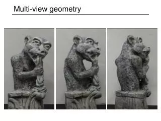

Multi-view geometry
E N D
Presentation Transcript
Multi-view geometry problems • Structure: Given projections of the same 3D point in two or more images, compute the 3D coordinates of that point ? Camera 1 Camera 3 Camera 2 R1,t1 R3,t3 R2,t2 Slide credit: Noah Snavely
Multi-view geometry problems • Stereo correspondence: Given a point in one of the images, where could its corresponding points be in the other images? Camera 1 Camera 3 Camera 2 R1,t1 R3,t3 R2,t2 Slide credit: Noah Snavely
Multi-view geometry problems • Motion: Given a set of corresponding points in two or more images, compute the camera parameters ? Camera 1 ? Camera 3 ? Camera 2 R1,t1 R3,t3 R2,t2 Slide credit: Noah Snavely
X? x2 x1 O2 O1 Structure: Triangulation • Given projections of a 3D point in two or more images (with known camera matrices), find the coordinates of the point
X? x2 x1 O2 O1 Structure: Triangulation • We want to intersect the two visual rays corresponding to x1 and x2, but because of noise and numerical errors, they don’t meet exactly
Triangulation: Geometric approach • Find shortest segment connecting the two viewing rays and let X be the midpoint of that segment X x2 x1 O2 O1
Triangulation: Linear approach Cross product as matrix multiplication:
Triangulation: Linear approach Two independent equations each in terms of three unknown entries of X
Triangulation: Nonlinear approach • Find X that minimizes X? P1X x2 x1 P2X O2 O1
Epipolar geometry X x x’ • Baseline – line connecting the two camera centers • Epipolar Plane – plane containing baseline (1D family) • Epipoles • = intersections of baseline with image planes • = projections of the other camera center • = vanishing points of the baseline (motion direction)
The Epipole Photo by Frank Dellaert
Epipolar geometry X x x’ • Baseline – line connecting the two camera centers • Epipolar Plane – plane containing baseline (1D family) • Epipoles • = intersections of baseline with image planes • = projections of the other camera center • = vanishing points of the baseline (motion direction) • Epipolar Lines - intersections of epipolar plane with image planes (always come in corresponding pairs)
Example: Motion perpendicular to image plane • Points move along lines radiating from the epipole: “focus of expansion” • Epipole is the principal point
Epipolar constraint • If we observe a point x in one image, where can the corresponding point x’ be in the other image? X x x’
Epipolar constraint X X X x x’ x’ x’ • Potential matches for x have to lie on the corresponding • epipolar line l’. • Potential matches for x’have to lie on the corresponding • epipolar line l.
Epipolar constraint: Calibrated case • Assume that the intrinsic and extrinsic parameters of the cameras are known • We can multiply the projection matrix of each camera (and the image points) by the inverse of the calibration matrix to get normalized image coordinates • We can also set the global coordinate system to the coordinate system of the first camera. Then the projection matrices of the two cameras can be written as [I | 0] and [R | t] X x x’
Epipolar constraint: Calibrated case X = (x,1)T x x’ = Rx+t t R The vectors Rx, t, and x’ are coplanar
Epipolar constraint: Calibrated case X x x’ Essential Matrix (Longuet-Higgins, 1981) The vectors Rx, t, and x’ are coplanar
Epipolar constraint: Calibrated case • E x is the epipolar line associated with x(l' = E x) • ETx'is the epipolar line associated with x'(l = ETx') • E e= 0 and ETe' = 0 • Eis singular (rank two) • E has five degrees of freedom X x x’
Epipolar constraint: Uncalibrated case • The calibration matrices K and K’ of the two cameras are unknown • We can write the epipolar constraint in terms of unknown normalized coordinates: X x x’
Epipolar constraint: Uncalibrated case X x x’ Fundamental Matrix (Faugeras and Luong, 1992)
Epipolar constraint: Uncalibrated case X x x’ • F xis the epipolar line associated with x(l' = F x) • FTx'is the epipolar line associated with x'(l' = FTx') • F e= 0 and FTe'= 0 • Fis singular (rank two) • F has seven degrees of freedom
Minimize: under the constraint||F||2=1 The eight-point algorithm
The eight-point algorithm • Meaning of errorsum of squared algebraic distances between points x’iand epipolar lines Fxi (or points xi and epipolar lines FTx’i) • Nonlinear approach: minimize sum of squared geometric distances
Problem with eight-point algorithm • Poor numerical conditioning • Can be fixed by rescaling the data
The normalized eight-point algorithm • Center the image data at the origin, and scale it so the mean squared distance between the origin and the data points is 2 pixels • Use the eight-point algorithm to compute F from the normalized points • Enforce the rank-2 constraint (for example, take SVD of F and throw out the smallest singular value) • Transform fundamental matrix back to original units: if T and T’ are the normalizing transformations in the two images, than the fundamental matrix in original coordinates is T’TF T (Hartley, 1995)
From epipolar geometry to camera calibration • Estimating the fundamental matrix is known as “weak calibration” • If we know the calibration matrices of the two cameras, we can estimate the essential matrix: E = K’TFK • The essential matrix gives us the relative rotation and translation between the cameras, or their extrinsic parameters