Download
1 / 25
250 likes | 279 Views
Learn about point estimates, errors of estimation, confidence levels, critical values, and creating confidence intervals for population parameters based on sample data.

E N D
Point Estimate an estimate of a population parameter given by a single number
Examples of Point Estimates • is used as a point estimate for .
Examples of Point Estimates • is used as a point estimate for . • s is used as a point estimate for .
Error of Estimate the magnitude of the difference between the point estimate and the true parameter value
Confidence Level • A confidence level, c, is a measure of the degree of assurance we have in our results. • The value of c may be any number between zero and one. • Typical values for c include 0.90, 0.95, and 0.99.
Critical Value for a Confidence Level, c the value zc such that the area under the standard normal curve falling between – zc and zc is equal to c.
– zc 0 zc Critical Value for a Confidence Level, c P(– zc < z < zc ) = c This area = c.
– z.90 0 z.90 Find z0.90 such that 90% of the area under the normal curve lies between z-0.90 and z0.90. P(-z0.90 < z < z0.90 ) = 0.90 .90
– z.90 0 z.90 Find z0.90 such that 90% of the area under the normal curve lies between z-0.90 and z0.90. • P(0< z < z0.90 ) = 0.90/2 = 0.4500 .4500
– z.90 0 z.90 Find z0.90 such that 90% of the area under the normal curve lies between z-0.90 and z0.90. • P( z < z0.90 ) = .5 + 0.4500 = .9500 .9500
Find z0.90 such that 90% of the area under the normal curve lies between z-0.90 and z0.90. • According to Table 5a in Appendix II, 0.9500 lies exactly halfway between two area values in the table (.9495 and .9505). • Averaging the z values associated with these areas gives z0.90 = 1.645.
Common Levels of Confidence and Their Corresponding Critical Values
Create a 95% confidence interval for the mean driving time between Philadelphia and Boston. Assume that the mean driving time of 64 trips was 6.4 hours with a standard deviation of 0.9 hours.
= 6.4 hourss = 0.9 hoursApproximate as s = 0.9 hours. 95% Confidence interval will be from
95% Confidence Interval: 6.4 – .2205 < < 6.4 + .2205 6.1795 < < 6.6205 We are 95% sure that the true time is between 6.18 and 6.62 hours.