Download
1 / 40
410 likes | 644 Views
Nearest Neighbor Queries Sung-hsun Su April 12, 2001. [1] Nick Roussopoulos, Stephen Kelley, Frederic Vincent: Nearest Neighbor Queries. SIGMOD Conference 1995: 71-79.

E N D
Nearest Neighbor QueriesSung-hsun SuApril 12, 2001 • [1] Nick Roussopoulos, Stephen Kelley, Frederic Vincent: Nearest Neighbor Queries. SIGMOD Conference 1995: 71-79. • [2] G. R. Hjaltason and H. Samet, Distance browsing in spatial databases, ACM Transactions on Database Systems 24, 2 (June 1999), 265-318.
Outline • Introduction to Nearest Neighbor Query • Spatial data structure – R-Tree • K-NN Algorithm in [1] • Incremental NN Algorithm in [2]
The Need of NN Query • Used when data have spatial property • Example: Geographical Info System, Astronomical Data • Spatial predicate Find the k nearest stars from the Earth Find the k nearest stars which is at least 10 LY away Find the nearest gas station in the east Find the furthest TCAT bus stop
Difficulties in NN Query • Need to scan the whole table if unordered • Spatial data structure: • 1D – Simply use a B+ tree or other sorted data structure • 2D or higher dimensional? - A sorted structure for all queries? No.
Data structure – First Trial • Need complex data structure • First trial – Fixed grids: Partition the space evenly into rectangles, cubes, … - Search the neighboring grids first - Distance to objects in a grid is bounded • Disadvantage?
Disadvantages of Fixed Grids • May still access many additional objects • Skewed data distribution • Grid size too large: inefficient search Grid size too small: waste of storage • Need some hierarchical and scalable data structure
Spatial Tree Structures • Make it possible to resolve cluster problem • Some Trees provide balanced structure • Insert/split dynamically • Good construction of trees will provide efficient search • Spatial Trees: K-D Tree, R-Tree, LSD-Tree, Quad-Tree … etc
A Glance of Algorithms • [1]: K-NN Query • Apply a modified DFS on R-Tree • [2]: Incremental NN Query • A Priority First Search on different kinds of spatial tree structure • Incremental • Distance browsing
R-Tree Introduction • Balanced structure, like B+Tree • Each node is an MBR (Minimal Bounding Rectangle) • A node minimally bounds all descendants • Non-leaf: (RECT, pointer to a child node) • Leaf: (RECT, pointer to an object) • Branching factor is chosen to fit a block or page
R-Tree Example Root Root B G C I J H A B C F K A D D E F G H I J K E Objects
Good and Bad R-Trees • Bad R-Tree: Contains much dead space • Good R-Tree: Minimize overlapped area • MBR estimates its objects better
Algorithms in [1] • Finding K Nearest Neighbors • Two metrics introduced: • MINDIST (optimistic) • MINMAXDIST (pessimistic) • Pruning • DFS Search
Space and Rectangle • Euclidean Space with n dimension: E(n) • A Rectangle is defined by R=(S,T), S, T are two points on a diagonal (r1, r2..rn), (t1, t2..tn) that: For all k=1 to n, tk>rk • Just simplifies computation
MINDIST(Optimistic) • MINDIST(RECT,q): the shortest distance from RECT to query point q • For all descendant (nodes/objects) in RECT, their distance to q is greater or equal than MINDIST(RECT,q) • This provides a lower bound for distance from q to objects in RECT • Use square of the distance as the metric
Calculation of MINDIST • MINDIST(P,R) = if if otherwise (between si and ti) T(t1, t2) (p1,p2) (r1,r2)=(t1,p2) y x S(s1, s2)
MINMAXDIST(Pessimistic) • MBR property: Every face (edge in 2D, rectangle in 3D, hyper-face in high D) of any MBR contains at least one point of some spatial object in the DB. • MINMAXDIST: Calculate the maximum dist to each face, and choose the minimal. • Upper bound of minimal distance • At least 1 object with distance less or equal to MINMAXDIST in the MBR
Illustration of MINMAXDIST (t1,t2) MINDIST (t1,p2) (p1,p2) MINMAXDIST y x (s1,s2) (t1,s2)
Calculation of MINMAXDIST • Can be done in O(n)
Pruning • MINDIST(M) > MINMAXDIST(M’) : • M can be pruned • Distance(O) > MINMAXDIST(M’) : • O can be discarded • MINDIST(M) > Distance(O) • M can be pruned
DFS Search on R-Tree • Traversal: DFS • Expanding Non-leaf: Order its children by the metrics (MINDIST or MINMAXDIST). Prune before/after visiting each child. • Expanding Leaf: Compare objects to the nearest neighbor found so far. Replace it if the new object is closer. • Not a straight-forward approach - make only local decision • May visit non-optimal objects before the NN is found. • Best first search: simple, and never visit non-optimal nodes.
Extending to K-NN • Maintain k nearest neighbors found so far. • Use the k-th furthest MBR/objects for pruning • Blocking algorithm. No pipelining.
Experimental Results • Real world data: TIGER, Satellite data • Synthetic data • R-Tree Construction: (branching factor=50) • Presorting data with Hilbert Number • Apply a packing technique • Branching factor is 50 • Performance measure: # of pages accessed
Experimental Results (Cont’d) • Linear with k (number of neighbors to find), but slowly. • Grow linear with height of the tree Log(size of data set) • MINDIST outperforms MINMAXDIST • 20% faster in general, 30% in dense data set • Reason: R-Tree is packed very well. MINDIST approaches actual minimal distance.
Problems with this algorithm • Nodes/objects are not visited by order of distance. Blocking • May access non-optimal objects, and discard/prune them. Not incremental • Need to know k in advance, no distance browsing, difficult to combine with other predicates.
Distance Browsing • To browse object in distance order • Example: Find the k nearest star with distance > 10LY • How to apply algorithm[1] to this query? • Select stars with distance >10LY first • Materialize the first result • And then build another R-Tree • What if selectivity is very high?
Solution to Distance Browsing • Very low selectivity (nearest city with 2M+ population) • Perform selection first, build an R-Tree, perform k-NN • Otherwise • Need incremental k-NN, pipeline the result to selection operator • Can stop at any time
Overview of algorithm in [2] • A generic algorithm for different spatial data structure and different distance definition. • Use Priority Queue to perform best first search using minimal distance(optimistic). • Ensure that no object/node is visited before another closer object/node.
Search Algorithm • Always expand the nearest node or object in the priority queue. • Treat objects special cases of nodes. • While expanding a node, calculate each children’s distances from query point, and add them into priority queue. • While expanding an object, just report it and then continue.
Requirement for Tree/Distance • Tree/Distance must conform the following rules: • Allow a node/object to have more than one parents • There may be duplicate of object pointer in the tree. • The region covered by a node must be completely contained within union of it parents’ region. • Consistence distance: For all query point q and node/object n, at least one of its parents, n’ has distance d(q,n’) <= d(q,n). (To ensure expanding nodes in order)
Remarks to Tree/Distance • Applicable tree: Quad-tree, R-Tree, R+-Tree, LSD-Tree, K-D-B Tree…etc • Applicable distance measure: Euclidean, Manhattan, Chessboard…etc • Almost of spatial trees don’t have duplicate nodes. A node is fully contained in its parent. • Some trees allow duplicate objects. We have to detect and remove duplicates. • R-Tree doesn’t have duplicates.
Example R=6 R=11 Root B F A D E C
Order of expansion R=0: Expand Root, { A[1],B[7] } R=1: Expand A, { D[1],B[7],C[10] } R=1: Expand D, { Circle[1],B[7],C[10] } R=1: Report Circle, { B[7], C[10] } R=7: Expand B, { E[8], C[10], F[12] } R=8: Expand E, { Rectangle[8], C[10], F[12] } R=8: Report Rectangle, { C[10], F[12] } R=10: Expand C, { F[12], Triangle[13] } R=12: Expand F, { Triangle[13], Moon[14] } R=13: Report Triangle, { Moon[14] } R=14: Report Moon, { }
Observation • All nodes/objects intersecting the search region(circle) are expanded, and their children are put in the queue. • All nodes/objects completely inside the search circle are already taken off the queue. • All nodes/objects completely outside the search circle are not examined. • It minimizes the number of objects to visit.
PseudoCode Queue=NewPriorityQueue(); EnQueue(Queue, Root, 0); While (NotEmpty(Queue)) { Element=Dequeue(Queue) If IsObject(Element) { /*Remove duplicate*/; Report(Element) } If IsLeaf(Element) { For each child object o, if Dist(o,Q)>=Dist(Element,Q) EnQueue(Queue,o,Dist(o,Q)); //Don’t need the comparison for R-Tree } If IsNonLeaf(Element) { For each child object o Enqueue(Queue,o,Dist(o,Q));} }
Variants • K Furthest: • Use MaxDist • Replace <= by >= • Distance selection: Select all stars between 15 LY and 20 LY. • Prune unqualified nodes • Pseudo code for search algorithm combining these 2 extension: Figure 5
Implementation of Priority Queue • Enough memory: Heap (minheap/maxheap) • Not enough: Use B+ Tree (sorted keep nodes with smaller distance in the memory) • Hybrid Scheme: Divide into 3 tiers. • Tier 1 uses in-memory heap. • Tier 2 is divided into several sections. Nodes in each sections are unordered bucket in memory, and the first bucket is moved to Tier 1 when Tier 1 is empty. • Tier 3 is stored on disk, and moved to memory when tier 1 and 2 is empty.
Theoretical Analysis • Assumption: Uniform distribution, 2D • Use the circular search region for analysis • K the area of search region • Number of leaf nodes in the priority queue circumference of search region = • Number of leaf nodes accessed = • Number of nodes accessed = • For non-uniform 2D case: very close to the result
Experimental Result • TIGER/Line file (17421~200482 segments) • Synthetic data (infinite random segments) • Construction: R* Tree • Distance Browsing: Inc-NN much faster than k-NN, the ratio increases at • Exact k-NN query: Inc-NN is 10~20% faster • Scalability: close to theoretical result • Very large k: k-NN can’t hold all k neighbors in memory
Conclusion • Inc NN outperforms other k-NN algorithms. • Inc NN enables distance browsing. • Number of node accesses (2D) is • Future work: • Compare this algorithm on different spatial structure • Investigate the behavior on very large data set where the PQ can’t fit into memory.