Download
1 / 19
190 likes | 475 Views
Nearest Neighbor and Reverse Nearest Neighbor Queries for Moving Objects. Simonas Šaltenis with Rimantas Benetis, Christian S. Jensen, Gytis Kar č iauskas. Nykredit Center for Database Research Department of Computer Science , Aalborg University. M otivation.

E N D
Nearest Neighbor and Reverse Nearest Neighbor Queries for Moving Objects Simonas Šaltenis with Rimantas Benetis, Christian S. Jensen, Gytis Karčiauskas • Nykredit Center for Database Research • Department of Computer Science, Aalborg University
Motivation • Position-aware, online, moving objects are enabled by the following trends. • Miniaturization of electronics • Advances in positioning systems (e.g., GPS, cellular infrastrucutre based systems) • Advances in wireless communications • Examples of position-aware online moving objects • 3G mobile-phones, as well as diverse types of personal digital assistants (online“cameras,” “wrist watches,” etc.) • Vehicles, including cars, public transportation, recreational vehicles, sea vessels, etc. • There is a need for a database support for storing and querying positions of large quantities of moving objects WIM workshop, Jyväskylä, August 4-7, 2002
Motivation – Sample LBSs • Location-aware advertising • Consumers may receive sales information for locations close to them. Here, the positional data is used together with an accumulated user profile to provide a better service. • Query: ”Find 5 cars closest to this gas station (as possible receivers of advertising).” • Location-aware, on-line games • Gamers “shoot” each other with their personal mobile devices. Suppose gamers can shoot only their nearest neighbor. • Query: “Find all gamers that have me as their nearest neighbor (so that I can attempt to avoid their fire).” • Ad-hoc mobile networks • Objects, which provide routing services to each other, may need to know who are their nearest neighbors and who has them as their nearest neighbors. WIM workshop, Jyväskylä, August 4-7, 2002
Outline • Motivation • Problem statement (data and queries) • NN queries • RNN queries • Summary WIM workshop, Jyväskylä, August 4-7, 2002
4 3 2 1 5 4 3 2 1 5 NN and RNN Queries • Nearest neighbor (NN) query – find an object(s) that is closest to a query point. • Reverse Nearest Neighbor (RNN) query – find objects that have a query point as their nearest neighbor. 4 3 2 1 5 WIM workshop, Jyväskylä, August 4-7, 2002
Problem Statement I • Data – a set of two-dimensional continuously moving points • To address continuous change, we represent the positions of points as functions of time, yielding time-parameterized positions. • We use linear functions to capture the present and future positions. • Function parameters are updated whenever an object deviates substantially from its predicted trajectory. • Given t0, the current and anticiapted, future position of a two-dimensional point is described by four parameters. WIM workshop, Jyväskylä, August 4-7, 2002
Problem Statement II • Query – a moving point q and a time interval [ts;te], where te ts current time. • Result – a subdivision of [ts;te] into non-intersecting intervals Tj. Each Tj is associated with a set of points that are nearest neighbors (reverse nearest neighbors) to q during Tj . For example: • RNNquery: (1, [0;5]) • Query result: (á{2, 5}, [0;3)ñ, á{2, 4}, [3;5]ñ) 4 4 3 3 2 2 1 1 5 5 WIM workshop, Jyväskylä, August 4-7, 2002
Outline • Motivation • Problem statement (data and queries) • NN queries • RNN queries • Summary WIM workshop, Jyväskylä, August 4-7, 2002
Result: p12 p12 p8 R1 R2 p8 p8 Query point R3 R4 R5 R6 R7 p12 p3 p4 p11 p5 p9 p10 p8 p6 p7 p12 p13 p1 p2 Pointers to data tuples NNs for Stationary Points I • Roussopoulos (1995) algorithm for R-trees, simplified by Cheung and Fu (1998) p6 R1 Candidate NN point: p8 Candidate NN point: Æ p7 p1 p4 R4 R3 p2 R5 p3 p5 R2 R7 p9 p13 p10 R6 p11 WIM workshop, Jyväskylä, August 4-7, 2002
NNs for Stationary Points II • The Rousopoulos algorithm performs a depth first search of the tree. Candidate NNs(CNNs) are maintained. • Whenever a node is visited • Pruning is performed: entries with bounding rectangles (R)with dist(R, q) larger than dist(CNN, q) are pruned. • Ordering is used when visiting the remaining entries of the node: entries with bounding rectangles with smaller dist(R, q) are visited first. WIM workshop, Jyväskylä, August 4-7, 2002
where A(t) is, e.g., the area of an MBR Time-Parameterized R-Tree • The TPR-tree (Šaltenis et al., 2000) is based on the R-tree. • Moving points are bounded with time-parameterized rectangles (TPBRs). • Min and max velocity coordinates are stored with each TPBR. • TPBRs are bounding from now on. • At any t > tcwe can get a valid R-tree: TPR-tree(t) = R-tree • Objects are grouped according to integrated R*-tree heuristics WIM workshop, Jyväskylä, August 4-7, 2002
NN Algorithm for the TPR-tree I • We “time-parameterize” the NN algorithm for R-trees, by observing how distance is time-parameterized: • Because the movements of points are described by linear functions, for any time interval [ts;te], the (square of) distance between these two points is a quadratic function dist(q,p)(t)= at2+bt+c, tÎ[ts;te]. • Similarly, any time interval [ts;te] can be subdivided into a finite (at most five) number of non-intersecting intervals so that, during each of the intervals, the (square of) distance between a point and a time-parameterized rectangle is a quadratic function. • Thus, finding out which point or TPBR is closer to the query point and during which time intervals (i.e., comparing two time-parameterized distances) involves solving one or several quadratic inequalities. dist=0 dist WIM workshop, Jyväskylä, August 4-7, 2002
NN Algorithm for the TPR-tree II • The time-parameterized NN algorithm has the same structure as the algorithm for the R-tree, but has modified pruning and ordering strategies. • Ordering: Entries of a node with the smallest metric are visited first (consider the average distance to the query point during the whole query time interval). • Pruning: The result list is initialized so that the distance from query point q to a candidate NN point (CNN) during the whole query time interval is infinite. Then, • Entries (both non-leaf and data) are pruned if the distance from them to q is greater than the distance from q to a CNN during the whole time interval. This involves checking each time-interval in the current result list. • If a data entry is not pruned, the time interval when it is closest to q is added to the result list. E.g., if the result list is (á{2}, [0;3)ñ, á{4}, [3;5]ñ) and, during [2;4), point 3 is closer to q than both 2 and 4, the result list is transformed to (á{2}, [0;2)ñ, á{3}, [2;4)ñ,á{4}, [4;5]ñ). Æ (dist = ¥) ts te cnn1 cnnn cnn2 ts te WIM workshop, Jyväskylä, August 4-7, 2002
Outline • Motivation • Problem statement (data and queries) • NN queries • RNN queries • Summary WIM workshop, Jyväskylä, August 4-7, 2002
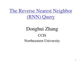
RNNs for Stationary Points • An algorithm for stationary points was proposed by Stanoi et al. (2000). • Idea: Let p be an NN of q among points in one of the six sectors Si. We call p an RNN candidate. Then, either q is the NN of p (and, thus, p is the RNN of q), or q has no RNNs in Si. There can be at most six RNNs – one for each Si. S2 • Sketch of the algorithm: • Run a restricted NNalgorithm in each Si, resulting in at most six RNN candidates. • To verify candidates, run the NNalgorithm with each candidate as the query point. x p S3 S1 60° q a b S4 S6 S5 WIM workshop, Jyväskylä, August 4-7, 2002
RNN Algorithm for the TPR-tree • Sketch of the algorithm • 1. For each of the sectors Si, run the NN algorithm to find a result list Bi. • 2. For each Biand for each element á{bk},Tkñ in Bi, calltheNN algorithm to check whether (and when) q is the NN of bkduring Tk. • Note that, in the NN algorithm, we can start a more aggressive pruning right away by setting q as a candidate NN of bk (instead of initially having an undefined candidate with an infinite distance). • Also, time interval TÌTk is excluded from consideration as soon as some point p is found that, during T, is closer to bkthan q. (Thus, we are sure that during Tbkis not an RNN of q). • The algorithm can be implemented so that only two top-down traversals of a tree are performed (steps 1 and 2). WIM workshop, Jyväskylä, August 4-7, 2002
RNNquery: (q, [0;2]): S2 S3 S1 q t =1 t =2 • á2, [1.5;2]ñ from B2 • á2, [1;1.5]ñ from B3 • Final answer: (á2, [1;2]ñ) RNN Example • Perform NN in S2: 7 • B2=(áÆ, [0;2]ñ) • B2=(á4, [0;2]ñ) 5 6 • B2=(á4, [0;1.5]ñ, á2, [1.5;2]ñ) 4 3 • Perform NN in S3: 2 • B3=(á2, [0;1.5]ñ, á3, [1.5;2]ñ) • Perform NN in S1: t =0 • B1=(á5, [0;2]ñ) • Check candidates in B1, B2 and B3: WIM workshop, Jyväskylä, August 4-7, 2002
Summary and Other Results • We provide the first algorithms for nearest neighbor and reverse nearest neighbor queries for continuously moving (data and query) points in a time interval. • NNalgorithm by Roussopoulos et al. is adapted. • RNNalgorithm by Stanoi et al. is adapted. • Persistent queries are supported – algorithms are provided that efficiently update the above-described result sets whenever a deletion or an insertion occurs before te. • Current-time continuous queries are supported by periodically computing and then maintaining the results of persistent queries. Balance is achieved between: • Maintaining too large query result (with a long future time interval) on each update operation • Performing too frequent queries (with short future time intervals) WIM workshop, Jyväskylä, August 4-7, 2002
Related Work • A lot of work has been done in NN query processing for stationary points in GIS and high-dimensional datasets (Roussopoulos et al., 1995, Hjaltason and Samet, 1999). • Kolios et al (1999) propose a solution for NN queries on one-dimensional moving points based on duality transformation. • The formulation of the problem is different (asks for one point that gets closest to the query point during the query time interval) • Song and Roussopoulos (2001) consider an NN problem where a query point is moving but data points are stationary. • Albers et al. (1998) consider how to maintain Voronoi diagrams of moving points. • Special index structures were proposed (Korn and Muthukrishnan, 2000, Yang and Lin, 2001) for the processing of RNN queries. WIM workshop, Jyväskylä, August 4-7, 2002