Download
1 / 21
210 likes | 222 Views
Learn about Confidence Intervals and Statistical Inference, how to estimate population parameters with intervals and interpret results effectively.

E N D
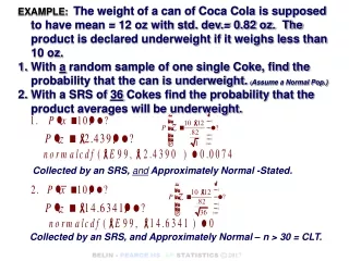
EXAMPLE:The weight of a can of Coca Cola is supposed to have mean = 12 oz with std. dev.= 0.82 oz. The product is declared underweight if it weighs less than 10 oz. • With a random sample of one single Coke, find the probability that the can is underweight. (Assume a Normal Pop.) • With a SRS of 36 Cokes find the probability that the product averages will be underweight. Collected by an SRS, and Approximately Normal -Stated. Collected by an SRS, and Approximately Normal – n > 30 = CLT.
25 c) 36 c) d)
CHAPTER 19 INTRODUCTION TO INFERENCE Statistical Inference – A method of Drawing Conclusions from data. The Two Types of Statistical Inference: I.Confidence Interval – This is a method of estimating the true value of the population parameter by constructing an interval that captures the true parameter
Margin of Error - The true population parameter is within m% of the sample estimate, with some degree of confidence.
Confidence Interval for Proportions Confidence Interval = Estimate ± Margin of Error
CONFIDENCE INTERVALS Confidence Level – A level C confidence interval for a parameter is an interval computed from sample data by a method that in repeated sampling has probability C of producing an interval containing the true value of the parameter. True Parameter An 85% Confidence Level
Interpreting 95% Confidence Interval We are 95% Confident that the true parameter (proportion) {add context here} will be captured by the constructed interval ( ). (based on one sample)
.453 .475 .498 .542 .565 .587 You ask 500 adults which of 2 candidates they support. = .52 are in favor your candidate. Sketch a 68-95-99.7 curve. Construct a 68% Confidence interval. Then Construct a 95% Confidence Interval. .52 I am 99.7%Confident that the true population proportion of votes in favor of my candidate is between 45.3% and 58.7%. I am 95%Confident that the true population proportion of votes in favor of my candidate is between 47.5% and 56.5%. I am 68%Confident that the true population proportion of votes in favor of my candidate is between 49.8% and 54.2%.
HW: PAGE 446: 1-5 He believes the true proportion of voters with a certain opinion is within 4% of his estimate. He believes the true percentage of children who are exposed to lead-base paint is within 3% of his estimate.
EXAMPLE: A large national company wants to keep costs down so it purchases fuel efficient vehicles. An SRS of 40 vehicles are selected and it is found that 28 of them are classified “Fuel Efficient”, what percent of the entire • company vehicles are fuel efficient? • 1. Estimate the population parameter with a 90% Confidence Interval and Interpret it. • 2. Estimate the population parameter with a 99% Confidence Interval and Interpret it. We can be 90% confident that the true population proportion of fuel efficient vehicles in the company is between 58.1% and 81.9%. We can be 99% confident that the true population proportion of fuel efficient vehicles in the company is between 51.3% and 88.7%.
Confidence Intervals for a Population Proportion: The Level C Confidence Interval for p-hat is computed by: To Interpret a Confidence Interval we say, “We can be 95% confident that the true population proportion is between a and b.”
What Does “85% Confidence” Really Mean? • The figure to the right shows that some of our confidence intervals capture the true proportion (the green horizontal line), while others do not:
Critical Value ( z* )– The number of standard deviation away from the mean with probability p lying to the right under the standard normal curve is called the Upper p critical value. C% P P -z* 0 z* Confidence Intervals for a Population Proportion: The Level C Confidence Interval for p-hat is computed by: where z* is the upper (1 – C)/2 critical value found by: z* = |INVNORM( (1 – C)/2 ) | or by Table.
Sampling Distribution of Pennies 150 – 125 – 100 – 75 – 50 – 25 – 0 – 142 66 27 21 1958 1963 1968 1973 1978 1983 1993 1998 2003 13 2008 1988 14 9 4 2 2 Penny’s Date