Solid Mechanics

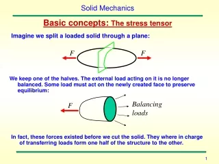
1. F F F Balancing loads Solid Mechanics Imagine we split a loaded solid through a plane: Basic concepts: The stress tensor We keep one of the halves. The external load acting on it is no longer balanced. Some load must act on the newly created face to preserve equilibrium: In fact, these forces existed before we cut the solid. They where in charge of transferring loads form one half of the structure to the other.

2. Unit normal to the facet Position Ai Solid Mechanics Imagine we are able to divide the surface in small facets and calculate the force acting on each one: • The stress is defined as the limit of the force per unit surface when the facets become infinitely small. • Stress is in fact a vector, not a scalar value. • One must realize that the force acting on a facet depends not only on its position, but also on its orientation. Two different cutting planes passing trough the same point would yield different values of the force.

3. tyx sy txy sx y sx x txy sy tyx Solid Mechanics In fact, the dependence of stress with orientation is a very simple function. Let’s start with a simple 2D example. Assume we have a square sheet under constant stress: It is common practice to split stresses in two components. The direct stress perpendicular to the face, and the shear stress which is tangent. s denotes direct stresses and t stands for shear. The first thing equilibrium tells us is that all the shear stresses have to be the same (otherwise, the part would start spinning):

4. y sx a txy x sy txy Solid Mechanics Now, if we cut the panel at a certain angle. What will be the stress on the new face? Force balance in x and y directions tells us: Please, observe that: So we can write:

5. Solid Mechanics For the more general 3D case we get the same expression: Remark that the stress tensor is always symmetric, so there are only six independent values on it. That is, the most general stress state on a point can be characterized with just six parameters. When we consider an arbitrary solid, the equilibrium condition is: For any volume W enclosed within a boundary G, bi being body forces and ti tractions on the boundary.

6. Solid Mechanics Using the divergence theorem, we can transform the equilibrium statement into: And since the control volume is arbitrary this implies: This is the strong form of the internal equilibrium equations. Remark that this is a set of three scalar equations, while the stress tensor contains six unknowns at each point. Therefore, this is not enough to solve a structural problem. We need a constitutive law relating stresses with strains. Note: The equation is also valid for the dynamic case if we include the inertial forces

7. Solid Mechanics We need a measure of the deformation of the material. We could use something as the velocity gradient tensor: Basic concepts: The strain tensor Note: The deformed (current) configuration coordinates of a point are denoted as xi, while the undeformed (reference) coordinates are usually referred to as Xi. The velocity gradient tensor can be used to calculate the relative velocity of two close points: However, we are not interested in rigid body motions as these do not cause stresses. We should subtract the spin rate from the velocity gradient to eliminate the rotation component.

8. y x gxy Solid Mechanics The components of the strain rate tensor are thus: When both strains and displacements are small we can integrate the strain rate to get the infinitesimal strain tensor: The direct components of the strain tensor represent stretches (increases in length per unit length) while the tangential components measure distortions (changes in angle between initially perpendicular lines)

9. Solid Mechanics The first invariant of the strain tensor is of particular significance: The volumetric strain measures the change of volume per unit volume. The strain tensor can be split into a deviatoric and a spherical part: Likewise, it is also possible to decompose the stress tensor. Its spherical part is called the hydrostatic stress:

10. Solid Mechanics When we deal with small enough strains, the behavior of most materials can be linearized. Thus, one could write: Basic concepts: Linear elastic materials This is called a linear elastic material because: • Stresses and strains are proportional (linear) • When strains are removed, the stresses return to zero (elastic) D being the fourth order elastic stiffness tensor. Given the symmetry of the stress and strain tensors, and the reciprocity principle not all the components are independent: So only 21 constants remain. Further, for the material to be stable, the strain energy stored as a result of deformation must be positive (otherwise it would blow-up on its own) thus:

11. Solid Mechanics Which means the stiffness matrix is positive definite. In many cases, on deals with (almost) isotropic materials. Then the stiffness tensor expression is greatly simplified and the behavior can be described with just two constants.From an uniaxial tension test we can derive the Young’s modulus: It turns out that even under those conditions, transversal strains develop. This is accounted for by means of Poisson’s ratio: For the case of multiaxial loading, we can calculate the total strain adding the different contributions,this is called the generalized Hooke’s law:

12. Solid Mechanics On the other hand, shear stresses are uncoupled form the rest so we can write: where the shear modulus can be written as: In many cases, we need the expression for the stresses as a function of strains. The previous relations can be inverted yielding: where the bulk modulus is:

13. Solid Mechanics INTERESTING FACTS In fluid dynamics, one tends to write: Which is quite similar to the previous expression, except for the fact that we use strain rates instead of strains. In fact (for the solid case) we could write: This being a very simple hypoelastic model (so simple, in fact, that there’s no point in using it). The important difference between the solid and the fluid case is that for a solid the instantaneous velocity field is not enough to calculate the stress tensor. Solids have memory, so the deformation history has to be integrated. Remark: As n approaches 0,5 the solid becomes incompressible. In fact, Poisson’s ratio must be less than 0,5 otherwise thermodynamics would break apart! Can you explain?

14. Solid Mechanics Using: The equations of linear isotropic elasticity we can write: And inserting this into the internal equilibrium statement yields: Or, if you prefer vector form:

15. Solid Mechanics Plus some boundary conditions: Of course, nobody solves these equations anymore. Enter the weak formulation; average over the domain the equilibrium condition: the test function representing in this case a virtual velocity field. Integrating by parts the stress term yields: As always, we can split the virtual velocity gradient:

16. Solid Mechanics Given that: We end up with the well known principle of virtual work: The power of the external loads equals the rate of work of internal equilibrating stresses (the strain rate is the energy conjugate of the Cauchy stress). The virtual work statement is at the core of the Finite Element Method. Given a displacement field depending on a finite number of parameters, the virtual work equation provides a systematic way to compute the solution. We build an approximate solution having this shape: Values of the approximate solution at control points (nodes) (supraindex j denotes value at node j) Interpolation functions

17. Solid Mechanics Therefore, the interpolation functions should satisfy: To make things even simpler, we divide the domain in small patches called “elements”. The nodes define the boundaries of the elements. We impose: With these restrictions, the calculations can be carried out on an elemental basis. Interpolation functions having these characteristics are called “shape functions”. The virtual velocity field can then be expressed as: Inserting this into the virtual work equation yields:

18. Solid Mechanics As the virtual displacements are independent, we could set all of them but one to zero and derive multiple equations. Let then As the stress tensor is symmetric, this is simply: Which, of course, we knew from the beginning, as this is the weak form of the equilibrium equations using the shape functions as test functions. This is a set of n (the number of nodes) equations for each space dimension. They can be solved for the nodal displacements if we write the stresses as a function of the nodal displacements.

19. Solid Mechanics While this may seem a bit confusing at first, it’s really easy. Let’s use the three node triangle as an example. Assuming we are dealing with plane strain conditions: Which is usually written in compact form as: For the stresses we have:

20. Solid Mechanics This can also be abbreviated as: therefore The strain energy density change due to a virtual displacement is then: The virtual work equation becomes: where

21. Solid Mechanics As the virtual displacement are arbitrary we can take one of them as unit and set the rest to zero. Furthermore, the nodal displacements are constant so they can be taken out of the integral. Thus: This system of equations is usually cast as: Generalized Nodal Displacements Generalized External Load Stiffness Matrix Remark that the differential work done by the external loads is:

22. Solid Mechanics Given that the work done by the external loads has to be stored as strain energy, the total strain energy in the system is: As the strain energy must be grater than zero whenever deformation takes place, the stiffness matrix is positive definite (except for underconstrained structures where rigid body motions are possible, in those cases the matrix is positive semidefinite). With this in mind, it is easy to see that the FEM solution satisfies the minimum total energy condition for the approximate solution: where F is the potential energy of the external loads

23. Solid Mechanics By introducing inertial forces we can account for the dynamic behavior without any major changes to the equations: Dynamic Problems the standard finite element interpolation can also be used for the acceleration The expression inside the parenthesis is called the “consistent” mass matrix

24. Solid Mechanics If we were to calculate the kinetic energy of the system, we would proceed this way: Which means the mass matrix is always positive definite. Most of the time the “lumped” mass matrix is used instead of the consistent form The use of the diagonal form entails no significant loss of accuracy and has the benefit of allowing explicit computation of the acceleration. To round things up, it is also possible to include a damping matrix: The shape of the equations is exactly the same as that found in the case of a simple harmonic oscillator, except this is a multiple degree of freedom system.

25. Solid Mechanics The undamped, free movement of a system is of special interest: Modal Dynamics We seek oscillatory solutions, so we try nodal displacements of the form: Therefore: This is a generalized eigenvalue problem, wi2 being the eigenvalues and fi the corresponding eigenvectors. An important property of the eigenvectors is that they are orthogonal with respect to the mass and stiffness matrices:

26. Solid Mechanics It is common practice to scale the eigenvectors to make them orthonormal with respect to the mass matrix then: If we build a matrix F such a generalized transform of coordinates is possible the system: becomes

27. Solid Mechanics if we multiply the last equation by FT we find something interesting As the eigenvectors are orthonormal the above simplifies to: where this means the equations for each mode are now uncoupled: with As one is usually interested in the response over a limited range of frequencies (in most cases the lower range) it is common practice to retain only a limited number of eigenmodes when solving the equations of motion. This is the basis of modal subspace dynamics.

28. L x P(x) P(x+dx) dM dx Solid Mechanics Given a uniform section rod, clamped on one end, calculate a couple of (axial) eigenmodes. An easy example Rod properties: • Young’s modulus E • Mass density r • Cross section A We shall first derive the analytical solution. If we consider an infinitesimal element along the beam, we can write the dynamic equilibrium equation:

29. Solid Mechanics So, we must solve: We also need a couple of boundary conditions. The clamped end cannot move so: while the other end is free (P=0) The solutions we seek have the form Therefore, the eigenvalue problem becomes:

30. Solid Mechanics The characteristic polynomial for the last equation is The function U is thus harmonic. Such a function subject to the constraints imposed by the boundary conditions must have the form: where The natural frequencies of the system (there’s an infinite number of them) are: Or, if you prefer Hz:

31. le ui ui+1 Solid Mechanics Now, let’s do it the FEM way. We’ll use the two node linear element which has just two degrees of freedom: The strain on the material is: So the stress becomes: The strain energy stored inside the element can be calculated as: Remember that: Which means:

32. Solid Mechanics For the mass matrix, we shall use the diagonal form. The kinetic energy of the element can be expressed as: If the element were to experience rigid body motion, its kinetic energy would be: Furthermore, as the bar is uniform the contribution of each node has to be the same; then: The elemental matrices we now have use the local element degrees of freedom. To build the global system of equations we must assemble them.

33. L n1 n2 n3 Solid Mechanics We will divide the rod in two equal length elements: Give me a break, I have to calculate everything by hand! The global stiffness matrix is: Likewise, we can assemble the mass matrix:

34. Solid Mechanics Remark the stiffness matrix is singular, this happens because the structure in unrestrained. We must impose the boundary conditions (u1=0 in this case). We end up with the system: Let: So the characteristic equation becomes: Then: It’s not too bad, theoretical value is p/2!