Download
1 / 25
250 likes | 465 Views
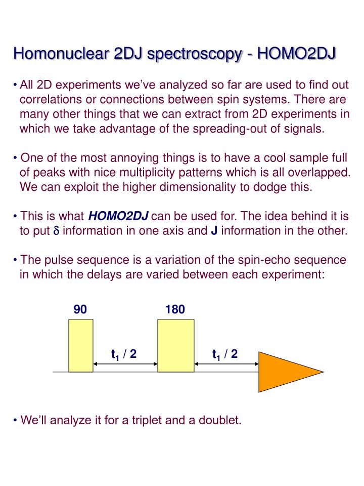
Homonuclear 2DJ spectroscopy - HOMO2DJ All 2D experiments we’ve analyzed so far are used to find out correlations or connections between spin systems. There are many other things that we can extract from 2D experiments in which we take advantage of the spreading-out of signals.

E N D
Homonuclear 2DJ spectroscopy - HOMO2DJ • All 2D experiments we’ve analyzed so far are used to find out • correlations or connections between spin systems. There are • many other things that we can extract from 2D experiments in • which we take advantage of the spreading-out of signals. • One of the most annoying things is to have a cool sample full • of peaks with nice multiplicity patterns which is all overlapped. • We can exploit the higher dimensionality to dodge this. • This is what HOMO2DJ can be used for. The idea behind it is • to put d information in one axis and J information in the other. • The pulse sequence is a variation of the spin-echo sequence • in which the delays are varied between each experiment: • We’ll analyze it for a triplet and a doublet. 90 180 t1 / 2 t1 / 2
HOMO2DJ - Triplet • Since the sequence is basically an homonuclear spin-echo, • we are refocusing chemical shifts irrespective of the t1 time. • For a triplet on-resonance with a coupling J, we have: • For different t1values, we get different pictures at the end: y y t1 / 2 90 x x y y t1 / 2 180 x x y y y x x x t1= 1 / 2J t1 ≈ 0 t1 > 1 / 2J
HOMO2DJ - Triplet (continued) • The center line will only decay due • to relaxation (T2). • The smaller components of the • triplet will vary periodically as a • function of the time t1 and the • J coupling: • In this case wo = 0, • because we are • on-resonance. • In the t2 (f2) dimension (the one corresponding to the • ‘real’ FID) we still have frequency information (the chemical • shifts of the multiplet lines). If we try to put it in an equation • of sorts: A(t1) = Ao * cos( J * t1) wo wo - J wo + J A(t1, t2) cos( J * t1) * trig( wo * t2 ) * trig( J * t2 )
HOMO2DJ - Triplet (…) • This is the whole process with real data for a triplet. First data • on t1 and f2 (after FT on t2): • FIDs obtained along - J, , y + J in t1, plus their • respective FTs: FT FT FT
HOMO2DJ - Triplet (…) • If we consider either the stack plot or the ‘pseudo’ equation, • a Fourier transformation in t2 and t1 will give us a 2D map • with chemical shift data on the f2 axis and couplings in the • f1 axis. Since we refocused chemical shifts during t1, all • peaks in the f1 axis are centered at 0 Hz: • Again, since we have different information in the f1 and f2 • dimensions, the 2D plot is not symmetric. • Now it’s easy to figure out what will happen to a doublet • with a coupling of J Hz, on-resonance (or not)… d (f2) J (f1) - J 0 Hz + J wo wo - J wo + J
HOMO2DJ - Doublet • After the 90 pulse and a certain time t1, the two magnetization • vectors will have dephased+ J / 2 * t1and - J / 2 * t1. For a • t1< 1 / 4J: • For different t1values, we would have a variation for the two • lines as a function ofcos( J / 2 * t1). • After FT in t1 and t2, the • 2D plot is the same, but • we have only two cross- • peaks... y y y t1 / 2 180 x x x d (f2) J (f1) - J / 2 0 Hz + J / 2 wo wo - J / 2 wo + J / 2
HOMO2DJ - Tilting • If we put the triplet and doublet together (either if they are • coupled to each other or not) we get: • Clearly, there is redundant information in the f2 dimension. • Since the peaks are skewed exactly 45 degrees, we can • rotate them that much in the computer and get them aligned • with the chemical shift. This is a tilting operation. J (f1) 0 Hz wod d (f2) wot J (f1) 0 Hz wod d (f2) wot
HOMO2DJ - Many signals • For a really complicated pattern we see the advantage. For a • 1H-1D that looks like this: • We have all the d information on the f2 axis and the J data on • the f1 axis. • We get an HOMO2DJ that has everything resolved in d’s • and J’s: d (f2) J (f1) 0 Hz
HOMO2DJ - Conclusion • Another advantage is that if we project the 2D spectrum • on its d axis, we basically get a fully decoupled 1H spectrum: • Finally, since we take ~ 256 or 512 t1 experiments, we have • that many points defining the J couplings which are between • 1 and 20 Hz. • For 50 Hz and 512 t1 experiments, 0.09 Hz / point. We can • measure JHH with great accuracy on the f1 dimension. d J 0 Hz
HOMO2DJ - Real data • This is for ethyl crotonate • at 400 MHz... • Note the resolution fot the multiplet at 5.7 ppm... No tilting... 2DJ 1D Tilted...
Heteronuclear 2D J spectroscopy • Last time we saw how we can separate chemical shift from • coupling constants in an homonuclear spectrum (1H) using a • 2D variation of the spin echo pulse sequence. • We basically modify the spin echo delays between • experiments to create the incremental delay. • We can do a very similar experiment, which also relies on • spin echoes, to separate 13C chemical shift and heteronuclear • J couplings (JCH).This experiment is called HETRO2DJ, and • the pulse sequence involves both 1H and 13C: • It’s basically the 2D version of APT... 90x 180y t1 / 2 t1 / 2 13C: 180y {1H} 1H:
Heteronuclear 2D J spectroscopy (…) • As we did last time, lets analyze what happens with different • types of carbons (a doublet and a triplet, i.e., a CH and a • CH2…). For a CH2: • The first 90 degree pulse puts things in the <xy> plane, were • the vectors start moving in opposite directions (again, we are • in resonance for simplicity…). • After the first half of the spin echo, we apply the 180 pulse on • carbons, which flips them back, and the 180 pulse on • protons, which, as we saw several times, inverts the labels of • the 13C vectors. y y a t1 / 2 90 x x b y y b a 180 (13C) 180 (1H) x x a b
Heteronuclear 2D J spectroscopy (…) • After the second half of the spin echo delay the vectors • continue to dephase because we have inverted the labels of • the protons. • Now, when we turn the 1H decoupler on, things become fixed • with respect to couplings, so any magnetization component • lying in the <y> axis cancels out. The components on the <x> • axis are not affected, and they will vary periodically with the • JCH coupling. For different t1’s we’ll get: y y b {1H} t1 / 2 x x a y y y x x x t1= 1 / 2J t1 ≈ 0 t1 = 1 / J
Heteronuclear 2D J spectroscopy (…) • What we see is that the signal arising from the center line will • not be affected. However, the two outer lines from the triplet • will have a periodic variation with time that depends in JCH. • If we we do the math, we will see that the intensity of what we • get in the t1 domain has a constant component (due to the • center line) plus a varying component (due to the smaller • components of the triplet): • Remember that • Acl = 2 * Aol • In the t2 (f2) dimension (the one corresponding to the real • FID) we still have frequency information (the chemical shifts • of the decoupled carbon). If we try to put it in an equation • of sorts: A(t1) = Acl + 2 * Aol * cos( J * t1) t1 = n / J t1 = n / 2J wo A(t1, t2) cos( J * t1) * trig( wo * t2 )
HETERO2DJ - Triplet (…) • If we consider either the stack plot or the ‘pseudo’ equation, • a Fourier transformation in t2 and t1 will give us a 2D map • with chemical shift data on the f2 axis and couplings in the • f1 axis. Since we refocused chemical shifts during t1, all • peaks in the f1 axis are centered at 0 Hz: • If we consider the equations and think of the different parts • we have, we can also see that we will have a constant • component (the center line) which will give us a frequency • on f1 of 0, plus a signal that varies with cos( JCH * t1 ), • which upon FT will give lines at +JCH and -JCH. • As oposed to homonuclear 2DJ spectroscopy in which we • had JCH information in both dimensions, we decoupled 1H • during acquisition, so we remove the JCH information from • the f1 axis. d (f2) J (f1) - J 0 Hz + J
HETERO2DJ - Doublet • We can do the same analysis for a doublet (and a quartet, • which will be almost the same…). • After the 90 degree pulse and the delay, the two vectors will • dephase as we’ve seen n-times... • As we had with the triplet, the two 180 pulses will invert the • vectors (13C pulse) and flip the labels (1H pulse). This means • that the two vectors will continue to dephase during the • second period (t1 / 2). y y a t1 / 2 90 x x b y y a b 180 (13C) 180 (1H) x x b a
HETERO2DJ - Doublet (continued) • Now, when we turn the 1H decoupler on, things become fixed • with respect to couplings. This is analogous to what • happened in the triplet… • If we just look at the signal we end up getting at different t1 • values, we get: • Note that in this case the ‘zero’ is at 1 / J because we the • vectors are moving ‘slower’ than for the triplet case (i.e., they • move at J / 2 * t instead of J * t...). y y b {1H} t1 / 2 x x a y y y x x x t1= 1 / J t1 ≈ 0 t1 > 1 / J
HETERO2DJ - Doublet (…) • If we look at the different slices we • get after FT in f2, we will see • something like this: • Here the signal will alternate • from positive to negative • at multiples of 1 / J... • If we do the second FT (in f1), we will get a 2D spectrum that • looks like this: t1 = n / J t1 = n / 2J wo d (f2) J (f1) - J / 2 • As for the triplet, we • don’t have couplings • in f2 (13C) because we • decoupled during the • t2 acquisition time. 0 Hz + J / 2 wo
HETERO2DJ - Conclusion • The main problem with this experiment is relaxation. Also, we • get the same information with a DEPT • in a fraction of the time. More ‘didactic’ • than anything else... • Done at 22 MHz with a home-brewed HETERO2DJ... CH2 CH
Separating the Wheat from the Chaff - Brief • introduction to phase cycling. • Usually even a single pulse experiment (90-FID) generates • more information that we bargained for. • Despite that we have only dealt with ideal spin systems that • only give ‘good’ signals, in the real world there are lots of • things that can appear in even a simple 1D spectrum that we • did not ask for. Some examples are: • Pulse length imperfections. A pulse is usually not ‘90’, so not • all the z magnetization gets tipped over the <xy> plane: z z f < 90 ‘90’y x x z y y x y
Phase cycling (continued) • Incorrect phases for the pulses. Instead of being exactly on • <x> or <y>, a pulse will be slightly dephased by an angle f: • Delay time imperfections. Artifacts of this type will result in • incomplete cancellation (or maximization) of signals in a • multiple pulse sequence like a spin-echo. • ‘White noise’ artifacts. Continuous frequency noise, that • generates a spike or peak at the same frequency all the time. • Vibrations. If the magnet vibrates (frequency), the probe will • vibrate, and we’ll see that in the spectrum... • All these things leave spurious signals in our 1D spectrum: • Spikes, wobbling baselines, side-bands, etc., etc. • As we go to higher dimensions, things get even nastier, • because, and completely consistent with Murphy’s Law, what • what we want to see decays or cancels out, and what we do • not care for grows… z z B1 90 ‘y’ x x f f y y
Phase cycling (…) • Lets say we have a pesky little signal at a certain frequency • that is there even when we have no sample in the tube (the • green peak...). This can originate from having a leak from a • circuit to the receiver coil, amplifiers, AD converter, etc. • More often than not, this frequency is exactly the carrier, or • the B1 frequency. Lets analyze a simple 90-FID sequence in • which this is happening (the red line is the receiver…): • If we repeat and acquire another FID, the spike will still be • there. It will also co-add with all other frequencies, and since • it is not random noise, it grows as we acquire more FIDs, just • like a real signal. • There is a real easy thing to do that will eliminate this type of • noise from a spectrum. It is based on the fact that we can • change our ‘point of view’ between experiments, while the • spike cannot. y 90y t1 (FID)x FT x wo wB1 wo
Phase cycling (…) • The procedure of changing our ‘point of view’ is called phase • cycling, and it involves shifting the phase of the pulses and/or • the receiver by a controlled amount between experiments. • In order to eliminate the spike, we do the following. We first • take an FID using a 90y pulse and the receiver in the <x> • axis just as shown in the previous slide. Then we shift the • phase of the 90 pulse by 180 degrees (90-y), and the receiver • also by 180 degrees to the <-x> axis (again, the red line…): • Now if we co-add the spectra (or FIDs), the signal at wB1 will • have alternating sign between successive scans, and it will • be canceled out after addition: y wo 90-y t1 (FID)-x FT wB1 x wo + = wB1 wo wB1 wo wo wB1
Phase cycling (…) • Instead of drawing all the vectors and frames every time we • refer to a phase cycle, we just use a shorthand notation. The • previous phase cycle can be written as: • In this case we only have one pulse and the receiver. In a • multiple pulse or 2D sequence we can extend this to all the • pulses that we need. • The previous sequence can be extended to the most common • phase cycling protocol used routinely, called CYCLOPS, • which is used with quadrature detection, and involves 4 cycles • instead of 2 (we have two receivers…): Cycle 90 Pulse Receiver 1 90 (y) 0 (x) 2 270 (-y) 180 (-x) Cycle 90 Pulse Rcvr-1 Rcvr-2 1 0 (x, 0) 0 (x, 0) 90 (y, 1) 2 90 (y, 1) 90 (y, 1) 180 (-x, 2) 3 180 (-x, 2) 180 (-x, 2) 270 (-y, 3) 4 270 (-y, 3) 270 (-y, 3) 0 (x, 0)
Phase cycling (…) • In a real pulse program the phase cycle is indicated at the • bottom. For a 13C spin echo (T2) experiment we have: • ;avance-version (GMB - 10/2004) • ;T2 measurement using Hahn spin-echo • ;with power gated decoupling • #include <Avance.incl> • "p2=p1*2" • "d11=30m" • "d12=20u" • 1 ze • 2 d12 pl13:f2 • d1 cpd2:f2 • d12 pl12:f2 • p1 ph1 • vd*0.5 • p2 ph2 • vd*0.5 • go=2 ph31 • d11 wr #0 if #0 ivd • lo to 1 times td1 • d11 do:f2 • exit • ph1=0 1 2 3 • ph2=0 3 2 1 • ph31=2 3 0 1 • ... • ... It is written as ‘rows’ instead of ‘columns’...