Chap6 Time Series Regression
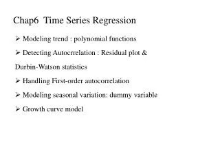
Chap6 Time Series Regression. Modeling trend : polynomial functions Detecting Autocrrelation : Residual plot & Durbin-Watson statistics Handling First-order autocorrelation Modeling seasonal variation: dummy variable Growth curve model. 6.1 Modeling trend. Y t = TR t + ε t ,.

Chap6 Time Series Regression
E N D
Presentation Transcript
Chap6 Time Series Regression • Modeling trend : polynomial functions • Detecting Autocrrelation : Residual plot & Durbin-Watson statistics • Handling First-order autocorrelation • Modeling seasonal variation: dummy variable • Growth curve model
6.1 Modeling trend Yt = TRt + εt , Trend : linear trend, curvilinear trend Model with polynomial trend Yt = TRt + εt = β0+ β1 t + β2 t2 …….+ βp t p+ εt , εt ~NID(0,σ2) Model with power trend Yt = β0( β1t ) εt , log(Yt) = logβ0+ log(β1 ) t +logεt logεt ~NID(0,σ2)
例6.1 No trend 例6.2 Linear trend 預測區間: for t =25
例6.3 Quadratic trend
6.2 Detecting autocorrelation 時序資料時常有自相關現象 自相關 (autocorrelation) -- 迴歸資料之誤差項依序列先後有相關性,此現象違背獨立性假設。 first-order autocorrelation:連續二資料間的相關性, 即εt 與 εt-1 間之相關性,一般假設此相關性與位置無關,只與時距有關,故對任一 t, ρ代表相關強度,ρ= cor(εt ,εt-1 ) for all t. 如何檢測出一階自相關? 1. 殘差圖,2. Durbin-Watson 檢定 (εt 與 εt-1 間相關,將反應在 et與 et-1間 )
自相關的檢定 -- Durbin-Watson Test Durbin-Watson 統計量: 註:1、 D ≒ 2(1-r1),0≦D≦4 4、SAS之 regression/linear 或 Times/arima 提供 D-W 值 2、檢定法則:依據 n, p, α在 TableA6查出 dL,α及 dU,α
正的自相關檢定 H0 :ρ= 0, H1 :ρ> 0 決策 • D < dL,α時,拒絕 H0 • D > dU,α時,不拒絕 H0 • dL,α <D < dU,α時,無法定論,(需要更多資料) ρ>0 ρ=0 ρ<0 0 dL dU 2 4-dU 4-dL 4 不確定區 臨界值
負的自相關檢定 H0 :ρ= 0,H1:ρ<0 決策 • (4-D) < dL,α時,拒絕 H0 • (4-D) > dU,α時,不拒絕 H0 • dL,α < (4-D) < dU,α時,無法定論,(需要更多資料) 注意: r1 >0 ,0< D < 2, r1 < 0 ,2< D < 4 r1 =ρ-hat
【例】 X:產品年銷售量(saleC) Y:某公司的年銷售量 (salei) 殘差圖 X-Y 分散圖
SAS/EG / regression/ linear 報表 (dL=1.2. dU=1.36) D=3.05 > 4-dL, 有負自相關現象,雖然R2值很高,得到的迴歸訊息是不正確的,需要修正模式。
資料的自相關現象對迴歸分析結果產生下列現象:資料的自相關現象對迴歸分析結果產生下列現象: • 係數的估計量仍為不偏,但無法達到最小變異數。 • MSE低估真實的誤差變異數。 • s.e.{bk}低估係數之標準差。 • t-test,F-test,及confidence interval 無法再直接應用。
6.6 First-order autocorrelative reg. model 如何修正含自相關現象的迴歸模式? 有多種方法,最常用的是 AR errors model, 即,假設迴歸式中的誤差項是一 AR(1) model. Model : Yt = β0 + β1 xt + εt , t= 1,2,…, n εt = ρ εt-1 + ut , |ρ|<1, ut ~NID(0,σ2) ρ為一階自相關係數,代表自相關程度之大小。 SAS-EG guide : Analyze → Time series → Reg. w Autoregressive Errors
共變異矩陣: 註 : 1、期望值=0 2、ρ愈大,影響愈遠。 3、若設εt = ρ1εt-1 + ρ2εt-2 + ut , 視為二階自相關模式AR(2)
【例】 X:產品年銷售量(saleC) Y:某公司的年銷售量 (salei) Reg. With Autoregressive Errors
估計: yt = 8.974 + 5.643 xt + εt , εt = -0.542εt-1
時間序列一階相關模式: Yt = TRt + εt , where εt = ρ εt-1 + ut , ut ~NID(0,σ2) 以Yule-Walker估計參數,βi, ρ 近似預測區間 (Prediction interval)
【Exc6.2】time series with linear trend (sale of watch) ρ-hat= 0.29, D=1.37, 無法定論自相關現象
時間序列一階自相關模式 預測區間
6.3 Seasonal variation 討論二種型態的季節變動 • Constant seasonal variation • Yt = TRt + SNt +ε t , (2) Increasing seasonal variation (Fig6.14) 可經由轉換變為第一型
(Fig6.14) 根號轉換後 Log 轉換後
6.4 Modeling seasonal variation 模式: Yt = TRt + SNt + εt , 以指標變數建模:S1~S11 代表11個月份的影響力,以第12個月為基底 Q1~Q3 代表3個季的影響力 如: Yt = TRt + SNt+εt = β0+β1t+β2M1+…+β12M11+εt,
[Exc6.4] Series with linear trend and increasing seasonal variation 步驟一、取 log 轉換,使季節原型固定 Y* = log (Y)
步驟二、建立含指標變數的迴歸式 模式: ln(Yt) = TRt + SNt+εt = β0+β1t+β2M1+…+β12M11+εt, where εt ~NID(0,σ2) ρ-hat= 0.39, D=1.19, 有自相關現象
步驟三、建立含AR(1) 誤差項的迴歸式 模式: ln(Yt) = TRt + SNt+εt = β0+β1t+β2M1+…+β12M11+εt, where εt = ρεt-1 + ut , ut ~NID(0,σ2) The AUTOREG Procedure
係數: εt = 0.39εt-1