Download
1 / 15
160 likes | 274 Views
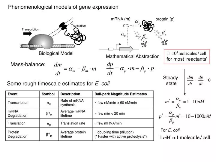
Phenomenological models of gene expression. Translation. mRNA (m). protein (p). Transcription. Biological Model. for most ‘reactants’. Mathematical Abstraction. Mass-balance:. Steady-state. Some rough timescale estimates for E. coli. Event. Symbol. Description.

E N D
Phenomenological models of gene expression Translation mRNA (m) protein (p) Transcription Biological Model for most ‘reactants’ Mathematical Abstraction Mass-balance: Steady-state Some rough timescale estimates for E. coli Event Symbol Description Ball-park Magnitude Estimates Transcription am Rate of mRNA synthesis ~ few nM/min < 60 nM/min mRNA Degradation b-1m Average mRNA lifetime ~ few min < 20 min Translation ap Translation rate ~ few mRNA/min For E. coli, Protein Degradation b-1p Average protein lifetime ~ doubling time (dilution) (* Faster with active proteolysis*)
R Transcriptional Repressor Slope: ‘Sensitivity’ or ‘Cooperativity’ ‘Capacity’ Idea: We use gR(r) to modify transcription rate: R Simple example – the autorepressor Recall: Transcriptional regulation Tells us how likely it is that RNAp will bind.
More interesting example – the toggle switch R1 R1 R2 R2 This is where the ‘circuit’ comes in Expect it to exist in two mutually exclusive states • If: • R1 is high, then R2 is low • R2 is high, then R1 is low What can we do with this? Coupled system of nonlinear differential equations…
Bistability Stable Equilibrium Points Exercise: The same with a) b) R1 R2 Unstable Equilibrium Point A R R3 What do you expect them to do? Write out a kinetic model. Simplification – Typically mRNA is short-lived, and protein is not. Assume mRNA attains steady-state very quickly compared to protein.
A In reality, molecule numbers are discrete. B B Changes are not infinitesimal – C(t) is not differentiable! A C C C ~ 10 C ~ 100 C ~ 1000 Assumes [C] is continuous and differentiable. Number of molecules of C ~ 1023 (mole)
Recall: For E. coli, for most ‘reactants’ Probability of being in state n at time t. n is the ‘inventory’ Instead of mass-balance, we use probability balance. Transition Probability Master Equation:
m-1 m m+1 Gain Loss Some notation : the step-operator Example – mRNA synthesis Difficult to solve! Mixes continuous time evolution with discrete state evolution.
Variance Mean-squared Mean Often we don’t need the whole distribution, just the moments IF the transition probabilities are linear, we can use moment generating function Subsequent derivatives of F give a linear combination of the moments of P: Turns a difference equation into a differential equation!
Fano factor for a Poisson process. (Fluctuations scale as ) Mean equal to variance is the footprint of a Poisson process. We can measure how close to Poisson a process is likely to be by the Fanofactor A dimensionless measure is the fractional deviation Exercise: Repeat the same analysis for unregulated protein expression. Find the steady-state fractional deviation in the protein number.
25 20 15 10 5 0 0 50 100 150 Number of b-Gal Molecules Time (min) Cai L, Friedman N, Xie XS (2006) Stochastic protein expression in individual cells at the single molecule level. Nature 440:358-362. Answer: ‘b’ is the burstiness of the process. It measures amplification of mRNA by translation ‘b’ is the average number of proteins translated from an errant transcript Remember: Moment generating functions only work if the transition probabilities are linear No dimerization, no feedback … No regulation!
Main approximation ideas – • Numerical simulation algorithms (Gillespie’s algorithm) • Direct simulation of a trajectory n(t) that conforms to the unknown distribution P(n,t) Perturbation schemes (van Kampen’s Linear Noise Approximation) Separate fluctuations from deterministic description using molecule number to scale. Stochastic description - Stoichiometry and propensity How fast? How much? Toggle switch example - Degradation Stoichiometry Matrix Synthesis
600 400 200 8 16 24 600 Five-times less molecules… State fairly localized about the stable points 160 400 120 80 200 40 8 16 24 200 400 600 Gillespie’s algorithm 1. Estimate when next reaction occurs, . 2. Estimate which reaction will occur, . 3. Update the system: Repeat…
comes from Poisson statistics Deterministic Concentration Fluctuations Linear noise approximation 1. Separate the deterministic evolution from the fluctuations 2. ‘Smooth-out’ the difference operator Reaction-rate equations Linear Fokker-Planck equation
Linear Fokker-Planck equation Reaction-rate equations Drift Diffusion Can show Dissipation Fluctuation For the variance Gaussian distribution ‘Fluctuation-dissipation’ relation
600 400 200 200 400 600 We can compare the two approaches, numerical and analytical • Numerical simulations work well: • few molecules, few reactions • quick overview • compelling pictures • Perturbation methods work well: • large system size (nearly deterministic) • more systematic exploration of parameters • analytic expression of moments • fluctuations in time-dependent (oscillatory) systems