Download
1 / 100
1.23k likes | 1.8k Views
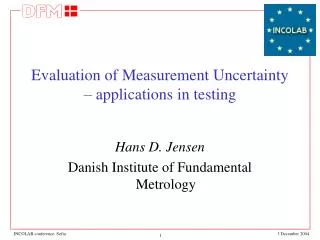
Evaluation of Measurement Uncertainty – applications in testing. Hans D. Jensen Danish Institute of Fundamental Metrology. Background. INCOLAB project Work Package 4 “Uncertainty as a generic activity” - Guide First draft available In this presentation topics from the guide:

E N D
Evaluation of Measurement Uncertainty – applications in testing Hans D. Jensen Danish Institute of Fundamental Metrology INCOLAB conference, Sofia
Background • INCOLAB project Work Package 4 “Uncertainty as a generic activity” - Guide • First draft available • In this presentationtopics from the guide: • Background on uncertainty • Tools for calculating • uncertainty • Examples along the way • DISCUSSION INCOLAB conference, Sofia
Outline • Why uncertainty? • Background and methods • Basic Philosophy • Measurement Model • Propagation of Uncertainties • Generic models • Basic measurement methods • The use of calibration curves • Handling test results • What is the measurand? • Physical models versus emperical models • Conclusions INCOLAB conference, Sofia
2,00 1,99 Why measurement uncertainty? • Measurement results, where the uncertainty is unknown, are basically useless! • They cannot be compared • They cannot be used for decision making • In daily life, we often often assume an uncertainty, but in measurement science uncertainty must be explicit! Will they fit? INCOLAB conference, Sofia
Max Not OK! Not OK? OK? OK! Min Not appropriate! Why uncertainty? • When making decisions based on measurement results, the uncertainty must be taken into account. INCOLAB conference, Sofia
Advantages by calculating uncertainty • Documentation for the declared uncertainty can be produced and shown to auditors, authorities, etc. • The critical elements in the measurement process can be identified • Quality control can be targeted the critical elements • Purchase of equipment can be optimised • Calibration of equipment can be optimised • Un-recognised sources of error can be revealed and new knowledge achieved INCOLAB conference, Sofia
Uncertainty in testing • A test procedure seeks to determine a “characteristic”, a property which helps to differentiate between items of a given population; Compliant/non-compliant, Good/bad, etc. • However, many physical tests rely on determining a quantitative result (an “indicator”), in order to specify the “characteristic”, e.g. limits, or is a quantitative characteristic itself. • Hence, the result of a test relies on a measurement result – and a measurement result is not complete without a statement of uncertainty INCOLAB conference, Sofia
Limits to uncertainty in testing • Measurement conditions (environment, specification of method and implementation) have great influence on the variability of the test results • If these are dominating, does it then make sense to evaluate measurement uncertainty? The problem is one of ‘division of labour!’ • Standards (norms) should ideally contain the expected uncertainty of the test result, given • The laboratory complies with the method (i.e. limits on influence factors are fulfilled) • The method is specified in sufficient detail • … however this is seldom the case INCOLAB conference, Sofia
Uncertainty in testing • The laboratory should • Demonstrate compliance with the test method, i.e. specification limits must be demonstrated fulfilled;this includes estimation of uncertainty • Demonstrate control of its basic measurements;this includes estimation of uncertainty • Demonstrate consistency with the variability of the test results with respect to recognised sources • The laboratory should not • Evaluate ‘method uncertainties’ of the test methods; this includes variability due to method test conditions • … this task lies with standardisation bodies, and the necessity may be revealed by intercomparison. INCOLAB conference, Sofia
“Method uncertainties” • For example, the glow-wire test method (application of a hot wire to insulation material to test for non-flammability, EN 60695) requires: • Wire diameter: (4,00 ± 0,04) mm; 0–10 % reduction • Maximum impact force: (1,0 ± 0,2) N • Maximum penetration: (7,0 ± 0,5) mm • Lab: (25 ± 10) °C, (60 ± 15) %RH • Contact time: (30 ± 1) s • Should the laboratory explore these limits with respect to the test result? • No; but demonstrate compliance with the limits! INCOLAB conference, Sofia
To note! • A keyword is Fit for purpose • Don’t overdo it, but don’t ignore it • Start simple – and with an eye on the requirements But, • A calculation is better than some loose, hand-waving arguments … (ask any technical assessor!) and • You might learn something about your measurement system… INCOLAB conference, Sofia
Basic Requirements The ideal method of evaluating uncertainty should be • universal, the method should be applicable to all kinds of measurement and all types of input data • internally consistent, the uncertainty should be derived from the components that contribute to it, independently of how the components are grouped or subdivided • transferable, it should be possible to use directly the uncertainty evaluated for one result as a component in evaluating the uncertainty of another measurement in which the first result is used INCOLAB conference, Sofia
Historical Background 1978: CIPM requests BIPM to address the uncertainty problem 1981: CIPM approves BIPM’s Recommendation INC-1 (1980) Expression of Experimentental Uncertainties 1986: CIPM requests member states to follow the recommendation 1993: ISO publishes Guide to the Expression of Uncertainty in Measurement (GUM) 1995: Eurachem makes guide for chemistry Uncertainty in testing is still under development(more in terms of application than in methods) INCOLAB conference, Sofia
”The method” INCOLAB conference, Sofia
BIPM Method • The value of a quantity, which is not known exactly, is considered as a random variable X. • The result of x of a measurement is an estimate of the expectation E(X). • The standard uncertainty u(x) is equal to the square root of an estimate of the variance V(X). • Type A: Expectations and (co)variances are estimated by statistical analysis of observations. • Type B: Expectations and (co)variances are calculated from assumed statistical distributions. INCOLAB conference, Sofia
What is a Random Variable? • A quantity that may take any value… with a given probability. • Described by a probability distribution given in the form of a Probability Density Function Why use random variablesfor uncertainty calculation? • ”Uncertainty” describes our insufficient knowledge – so does probabilities • We can use the body of knowledge from statistics and probability theory INCOLAB conference, Sofia
Quantities as Random Variables • Some valuesxof the quantity X are more likely than others INCOLAB conference, Sofia
E(X) Parameters of a Random Variable Relativeoccurance • The expectation, E(X):(the mean)The value that divides alloutcomes in two equalparts. • The variance, V(X):The expectation (the mean) of the square of the difference to the mean, V(X) = E((X – E(X))²) • The expectation is not necessarily the middle or the most probable value • The variance is a measure of the square of the “width" of the distribution INCOLAB conference, Sofia
60.4824 Repeatability • Example: A display with an indication I This could be the temperature measured by a sensor, a voltage or any other representation of a physical variable or simply the result of some complex measurement indicated by the instrument. INCOLAB conference, Sofia
reading Temperature number (°C) 1 60.4824 2 60.5164 3 60.5315 4 60.5466 5 60.5579 Repeatability If we repeat the measurement several times, we find that the readings are not identical. Five subsequent readings could yield results as shown in table and histogram.
More repetitions As the number of repetitions increases, the distribution of results approaches a limiting distribution. This limiting distribution reflects the maximum knowledge we can have about the measured quantity.
Normal distribution Based on many, independent (microscopic) contributions INCOLAB conference, Sofia
Normal distribution • The Normal distribution has the probability density function: • It is described fully by two parameters: μ and σ • The expectation is E(X) = μ • The variance is V(X) = σ² • The interval μ ± 2σ covers 95 % out the outcomes. INCOLAB conference, Sofia
X1 X2 Rules for calculation of variances • Scaling of a random variable X: • Addition of random variables X1 and X2: • Covariance: Interdependence of X1 and X2 E.g., if X2 ~ X1 X1–X2 INCOLAB conference, Sofia
Uncertainty • All measurements are subject to uncertainty — that may be from a dispersion of results or from insufficient knowledge • Hence, we must enter a state of mind, where we ”question” any numerical quantity used in our measurement • I.e. • The number I read on the display • The value I get from the label • The nominal value of a thermoelectric constant • The ability to repeat exactly any procedure INCOLAB conference, Sofia
BIPM Method • The value of a quantity, which is not known exactly, is considered as a random variable X. • The result of x of a measurement is an estimate of the expectation E(X). • The standard uncertainty u(x) is equal to the square root of an estimate of the variance V(X). • Type A: Expectations and (co)variances are estimated by statistical analysis of observations. • Type B: Expectations and (co)variances are calculated from assumed statistical distributions. INCOLAB conference, Sofia
Type A evaluation - Example Repeated observations of a quantity Q Observations: Average: Experimental variance: Degrees of freedom: Standard uncertainty: (… and of average) INCOLAB conference, Sofia
1 versus n observations It is important to distinguish between uncertainty of one observation and that of the average of observations One observation: q n observations: q1, q2, …, qn INCOLAB conference, Sofia
Uncertainty of standard deviations Assume: and INCOLAB conference, Sofia
Expanded uncertainty • For the Normal distribution, the interval μ ± 2σ covers 95 % of the outcomes, a confidence level which often is sufficient for decision making. • However, q ± 2 s does not cover 95 % of the outcomes, due to the uncertainty of s,due to the ‘few’ observations. INCOLAB conference, Sofia
Expanded uncertainty • We seek a factor k such that the intervalq – k s < x < q + k scovers 95 % of the outcomes. • The factor k is found from the Student’s t-distribution • The quality of the estimate s of σ is signified by the degrees of freedom; for the standard deviation it isn = n – 1. INCOLAB conference, Sofia
Reporting Result of a Measurement • With the appropriate coverage factor, we calculate the expanded uncertainty as • U = ku(remember, here we had u = s) • The result of a measurement are stated in a certificate in the form: • U are given with at most 2 significant digits; xis rounded accordingly. • Example: • Relevant to state k as well. INCOLAB conference, Sofia
Pooling of Variances • Assume that we have n experimental (relative) variances si2, which are estimates of the same (relative) variance s2. • Each experimental variance si2 has a (small) number of degrees of freedom ni. • The weighted average (pooled variance) of the experimental variances • is an estimate of s2 with np degrees of freedom. INCOLAB conference, Sofia
From Type A Evaluation ... • Example: A digital display with an indication I If the indication varies on the last decimals, e.g. ...25, …14, …47, …33, …29, …41, …13, …28, …40 the average and standard deviation are calculated: • But what if the last two digits were not shown in the display? What is then the uncertainty of the indication? 1.2125 INCOLAB conference, Sofia
P “1.20” “1.21” “1.22” Indication prior to rounding 1.200 1.205 1.210 1.215 ... to Type B Evaluation • No variation in indication Iis observed, but the uncertainty of the indication is not zero. • The uncertainty is estimated from an assumed distribution of the indication prior to rounding in the display! 1.21 INCOLAB conference, Sofia
Assumed distributions • This distribution is the Rectangular or Uniform distribution. • It is characterised by an upper and a lower limit, a and b. Often the symbol U(a,b) is used. • It is used when we assume (as our best estimate), the the magnitude of the quantityis between the limits, with equal probability. • ForU(a,b) we have: Expectation E(X) = (a + b) / 2 Variance V(X) = (b – a)2 / 12Remember:x = E(X), with standard uncertainty u(x) = INCOLAB conference, Sofia
Rectangular distribution Other examples for the Rectangular distribution: • Readings of an analog scale • Reference data from a handbook • Manufacturers specification for equipment • Estimate/experience med maximum variation Situations, where there are fixed limits and it is appropriate to assume equal probability for a value to appear in the interval. • If all else ‘fails’, use rectangular distribution! INCOLAB conference, Sofia
Type B Evaluation – in general • Assume a statistical frequency distribution f(x) for for the quantity X. • Calculate expectation and variance: • Standard uncertainty: INCOLAB conference, Sofia
Type B Evalution - Example Rectangular (uniform) distribution U(a,b) f(x) x a b INCOLAB conference, Sofia
f(x) x a b Type B Evaluation - Example Triangular distribution T(a,b) INCOLAB conference, Sofia
f(x) x a b Type B Evaluation - Exampel U-shaped distribution G(a,b) INCOLAB conference, Sofia
f(x) x -a a f(x) x -a a f(x) x -a a Type B Evaluation - Résumé U-shaped: Rectangular: Triangular: INCOLAB conference, Sofia
with Special Type B - samples • If one takes a sample of n units and finds x “red”, the estimate of the fraction of “red” equals INCOLAB conference, Sofia
Type B - Poisson • Discrete objects in a continuous “space”e.g. cars on a road, bacteria in a sausage, counts, … • With a constant density, the objects will be Poisson distributed • If we observe the number N, we get • Expectation value: xp = N • Variance: V(xp ) = N • And hence standard uncertainty: u(xp) = ÖN INCOLAB conference, Sofia
Assigning uncertainties • With the two basic tools,statistical evaluation (type-A) assigned distributions (type-B)we may take each of the quantities that enter our measurement problem, and quantity their value and their uncertainty INCOLAB conference, Sofia
calibrationbore built-inthermometer 180.02 ac resistance bridge working standard:Pt-100 sensor block calibrator Temperature block calibrator at 180 °C 180.0 INCOLAB conference, Sofia
Contributions we can think of tX actual temperature in the calibration bore tS temperature read from bridge (using pt100 calibration) tS correction due to uncertainty on resistance measurement tD correction due to drift of sensor since last calibration tiX correction due to setability of the built-in thermometer tRcorrection due to radial temperature inhomogeneity tAcorrection due to axial temperature inhomogeneity tHcorrection due to hysteresis effects tVcorrection due to temperature instability during measurements INCOLAB conference, Sofia
Individual contributions (1) • tSThe relation between temperature and resistance for the Pt-100 sensor is given in the certificate. The measured resistance corresponds to a temperature of 180.02 °C. The expanded uncertainty is given as U = 30 mK with a coverage factor k = 2. Mixed distribution Expectation value 180.02 °C Standard uncertainty u = 15 mK • tS Note that the uncertainty given above is the uncertainty on the temperature if the resistance is exactly known. However, there is also an uncertainty on the resistance measurement, which translates into an additional uncertainty on the temperature. We assume Expectation value: 0 °C Standard uncertainty: 10 mK INCOLAB conference, Sofia
Individual contributions (2) • tD From experience, the drift of the temperature since last calibration due to resistance ageing, is estimated to be within ± 40 mK. Rectangular distribution Expectation value 0 °C Standard uncertainty u = 20/3 mK • tiX The built-in thermometer has a resolution of 0.1 K Rectangular distribution Expectation value: 0 °C Standard uncertainty: 50/3 mK • tRThe radial temperature difference between the built-in thermometer and the calibration bore is estimated to be within ± 100 mK. Rectangular distribution Expectation value: 0 °C Standard uncertainty: 100/3 mK INCOLAB conference, Sofia
Individual contributions (3) • tA The axial temperature difference between the built-in thermometer and the calibration bore is estimated to be within ± 250 mK. Rectangular distribution Expectation value: 0 °C Standard uncertainty: 250/3 mK • tH From readings of tX during measurement cycles where the temperature is either increased or decreased, the uncertainty due to hysteresis is estimated to be within ± 50 mK Rectangular distribution Expectation value: 0 °C Standard uncertainty: 50/3 mK • tV Temperature variations during a 30 minute measurement cycle are estimated to be within ± 30 mK. INCOLAB conference, Sofia