Binary Search Trees
Binary Search Trees. Berlin Chen 陳柏琳 台灣師範大學資工系 副教授 參考資料來源: http://www.csie.ntu.edu.tw/~ds/. Binary Search Tree. Binary search tree Every element has a unique key The keys in a nonempty left subtree ( right subtree ) are smaller ( larger ) than the key in the root of subtree

Binary Search Trees
E N D
Presentation Transcript
Binary Search Trees Berlin Chen 陳柏琳 台灣師範大學資工系 副教授 參考資料來源: http://www.csie.ntu.edu.tw/~ds/
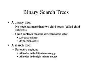
Binary Search Tree • Binary search tree • Every element has a unique key • The keys in a nonempty left subtree (right subtree) are smaller (larger) than the key in the root of subtree • The left and right subtrees are also binary search trees • A recursive definition! 60 30 20 70 40 25 5 12 80 65 22 2 15 10
Searching a Binary Search Tree tree_pointer search(tree_pointer root, int key) { /* return a pointer to the node that contains key. If there is no such node, return NULL */ if (!root) return NULL; if (key == root->data) return root; if (key < root->data) return search(root->left_child, key); return search(root->right_child,key); } Each tree node: - A key value (data) - Two pointers to it left and right children Complexity: O(h) A Recursive Version
Searching a Binary Search Tree tree_pointer search2(tree_pointer tree, int key) { while (tree) { if (key == tree->data) return tree; if (key < tree->data) tree = tree->left_child; else tree = tree->right_child; } return NULL; } A Iterative Version
Searching a Binary Search Tree • Search by rank permitted if • Each node have an additional field LeftSize which is 1 plus the number of elements in the left subtree of the node tree_pointer search3(tree_pointer tree, int rank) { while (tree) { if (rank == tree->LeftSize) return tree; if (rank < tree-> LeftSize) tree = tree->left_child; else { rank-= tree->LeftSize; tree = tree->right_child; } } return NULL; } 3 30 2 40 5 1 1 2
Insert Node in Binary Search Tree 30 30 30 40 5 40 40 5 5 80 35 2 80 2 2 Insert 35 Insert 80
Insertion into A Binary Search Tree void insert_node(tree_pointer *node, int num) {tree_pointer ptr, temp = modified_search(*node, num); if (temp || !(*node)) { ptr = (tree_pointer) malloc(sizeof(node)); if (IS_FULL(ptr)) { fprintf(stderr, “The memory is full\n”); exit(1); } ptr->data = num; ptr->left_child = ptr->right_child = NULL; if (*node) if (num<temp->data) temp->left_child=ptr; else temp->right_child = ptr; else *node = ptr; } } // Return last visited tree node // Not NULL
Deletion for A Binary Search Tree • Delete a leaf node • The left (or right) child field of its parent is set to 0 and the node is simply disposed 30 30 Delete 80 30 Delete 35 40 5 40 5 40 5 2 80 2 80 35 2
Deletion for A Binary Search Tree • Delete a nonleaf node with only one child • The node is deleted and the single-child takes the place of the disposed node 30 30 Delete 5 40 40 2 5 80 80 35 35 2
Deletion for A Binary Search Tree • Delete a nonleaf node with only one child 1 1 T2 T1 2 X T1 T2
Deletion for A Binary Search Tree • Delete a nonleaf node that has two children • The largest element in its left subtree or the smallest one in the right tree will replace the disposed mode 35 30 5 Delete 30 40 or 2 40 40 2 5 80 80 35 80 35 2
Deletion for A Binary Search Tree • Delete a nonleaf node that has two children • Recursive adjustments might happen 40 40 55 60 20 20 70 30 50 70 10 30 50 10 52 45 55 45 52 After deleting 60 Before deleting 60
Exercise • Implement a binary search which is equipped with • Insertion operation • Search operation • Search by key • Search by Rank • Deletion operation
A C B D E F G H K J I Trie A B D C E H F G I J K Trie Tree struct DEF_TREE { int Key; struct Tree *Child; struct Tree *Brother; struct Tree *Father; };
Graphs Berlin Chen 陳柏琳 台灣師範大學資工所 助理教授 參考資料來源: http://www.csie.ntu.edu.tw/~ds/
Definition • A graph G consists of two sets • A finite, nonempty set of vertices V(G) • A finite, possible empty set of edges E(G) • G(V,E) represents a graph • An undirected graph (graph) is one in which the pair of vertices in a edge is unordered, (v0, v1) = (v1,v0) • A directed graph (digraph) is one in which each edge is a directed pair of vertices, <v0, v1> != <v1,v0> tail head
Examples for Graph 0 0 0 1 2 1 2 1 3 3 6 5 4 G1 2 G2 complete graph incomplete graph G3 V(G1)={0,1,2,3} E(G1)={(0,1),(0,2),(0,3),(1,2),(1,3),(2,3)} V(G2)={0,1,2,3,4,5,6} E(G2)={(0,1),(0,2),(1,3),(1,4),(2,5),(2,6)} V(G3)={0,1,2} E(G3)={<0,1>,<1,0>,<1,2>} complete undirected graph: n(n-1)/2 edges complete directed graph: n(n-1) edges
Complete Graph • A complete graph is a graph that has the maximum number of edges • For undirected graph with n vertices, the maximum number of edges is n(n-1)/2 • For directed graph with n vertices, the maximum number of edges is n(n-1) • Example: G1 is a complete graph 0 1 2 3 G1 complete graph
Adjacent and Incident • If (v0, v1) is an edge in an undirected graph • v0 and v1 are adjacent • The edge (v0, v1) is incident on vertices v0 and v1 • If <v0, v1> is an edge in a directed graph • v0 is adjacent to v1, and v1 is adjacent from v0 • The edge <v0, v1> is incident on v0 and v1 0 1 0 1 2 2 G3 3 6 5 4 G2
Loop and Multigraph • Example of a graph with feedback loops and a multigraph (Figure 6.3) • Edges of the form (v, v) or <v, v> : self edge or self loop 0 0 2 1 3 1 self edge multigraph: multiple occurrences of the same edge (a) 2 (b)
Subgraph and Path • A subgraph of G is a graph G’ such that V(G’) is a subset of V(G) and E(G’) is a subset of E(G) • A path from vertex vp to vertex vq in a graph G, is a sequence of vertices, vp, vi1, vi2, ..., vin, vq, such that (vp, vi1), (vi1, vi2), ..., (vin, vq) are edges in an undirected graph • The length of a path is the number of edges on it
Figure 6.4: subgraphs of G1 and G3 0 1 2 0 0 3 1 2 1 2 3 0 0 0 0 1 1 1 2 2 0 1 2 3 (i) (ii) (iii) (iv) (a) Some of the subgraph of G1 G1 0 單一 分開 1 (i) (ii) (iii) (iv) (b) Some of the subgraph of G3 2 G3
Simple Path and Cycle • A simple path is a path in which all vertices except possibly the first and the last are distinct • A cycle is a simple path in which the first and the last vertices are the same • In an undirected graph G, two vertices, v0 and v1, are connected if there is a path in G from v0 to v1 • An undirected graph is connected if, for every pair of distinct vertices vi, vj, there is a path from vi to vj
connected 0 0 1 2 1 2 3 3 6 5 4 G1 G2 tree (acyclic graph)
Connected Component • A connected component of an undirected graph is a maximal connected subgraph • A tree is a graph that is connected and acyclic • A directed graph is strongly connected if there is a directed path from vi to vj and also from vj to vi • A strongly connected component is a maximal subgraph that is strongly connected
H2 H1 0 4 1 2 5 3 6 7 G4(not connected) Figure 6.5: A graph with two connected components connected component (maximal connected subgraph)
Figure 6.6: Strongly connected components of G3 strongly connected component (maximal strongly connected subgraph) not strongly connected 0 2 0 1 1 2 G3
Degree • The degree of a vertex is the number of edges incident to that vertex • For directed graph, • the in-degree of a vertex v is the number of edgesthat have v as the head • the out-degree of a vertex v is the number of edgesthat have v as the tail • if di is the degree of a vertex i in a graph G with n vertices and e edges, the number of edges is
undirected graph degree 0 3 0 2 1 2 1 2 3 3 3 3 3 6 5 4 3 3 1 G1 1 1 1 G2 0 in:1, out: 1 directed graph in-degree out-degree in: 1, out: 2 1 in: 1, out: 0 2 G3
ADT for Undirected Graph structure Graph is objects: a nonempty set of vertices and a set of undirected edges, where each edge is a pair of vertices functions: for all graph Graph, v, v1 and v2 Vertices Graph Create()::=return an empty graph Graph InsertVertex(graph, v)::= return a graph with v inserted. v has no incident edge Graph InsertEdge(graph, v1,v2)::= return a graph with new edge between v1 and v2 Graph DeleteVertex(graph, v)::= return a graph in which v and all edges incident to it are removed Graph DeleteEdge(graph, v1, v2)::=return a graph in which the edge (v1, v2) is removed Boolean IsEmpty(graph)::= if (graph==empty graph) return TRUE else return FALSE List Adjacent(graph,v)::= return a list of all vertices that are adjacent to v
Graph Representations • Adjacency Matrix • Adjacency Lists • Adjacency Multilists
Adjacency Matrix • Let G=(V,E) be a graph with n vertices. • The adjacency matrix of G is a two-dimensional n by n array, say adj_mat • If the edge (vi, vj) is in E(G), adj_mat[i][j]=1 • If there is no such edge in E(G), adj_mat[i][j]=0 • The adjacency matrix for an undirected graph is symmetric; the adjacency matrix for a digraphneed not be symmetric
4 0 1 5 2 6 3 7 Examples for Adjacency Matrix 0 0 1 2 3 1 2 G2 G1 symmetric undirected: n2/2 directed: n2 G4
Merits of Adjacency Matrix • From the adjacency matrix, to determine the connection of vertices is easy • The degree of a vertex is • For a digraph, the row sum is the out_degree, while the column sum is the in_degree sum up a row sum up a column
Data Structures for Adjacency Lists Each row in adjacency matrix is represented as an adjacency list #define MAX_VERTICES 50 typedef struct node *node_pointer; typedef struct node { int vertex; struct node *link; }; node_pointer graph[MAX_VERTICES]; int n=0; /* vertices currently in use */
4 0 1 2 5 6 3 7 0 1 2 3 0 1 2 3 1 1 2 3 2 0 1 2 3 4 5 6 7 0 2 3 0 3 0 1 3 0 3 1 2 1 2 0 5 G1 0 6 4 0 1 2 1 5 7 1 0 2 6 G4 G3 2 An undirected graph with n vertices and e edges ==> n head nodes and 2e list nodes
Interesting Operations • Degree of a vertex in an undirected graph • Number of nodes in adjacency list • Number of edges in a graph • Determined in O(n+e) • Out-degree of a vertex in a directed graph (digraph) • Number of nodes in its adjacency list • In-degree of a vertex in a directed graph (digraph) • Traverse the whole data structure • Or maintained in inversed adjacency lists
0 4 1 2 5 3 6 7 Compact Representation node[0] … node[n-1]: starting point for vertices node[n]: n+2e+1 (upper bound of the array) The vertices adjacent from vertex i are stored in array indexed from node[i] to node[i+1]-1 4 0 5 1 6 2 7 3
Inverse Adjacency Lists Figure 6.10: Inverse adjacency lists for G3 0 1 NULL 0 1 2 0 NULL 1 1 NULL 2 Determine in-degree of a vertex in a fast way.
tail head column link for head row link for tail Figure 6.11: Alternate node structure for adjacency lists • A simplified version of the list structure for sparse matrix representation for out-degree information for in-degree information Information for an edge
0 1 2 1 0NULL 0 1 NULLNULL 1 2 NULLNULL 2 NULL 1 0 Figure 6.12: Orthogonal representation for graph G3 head nodes (shown twice) 0 1 2
1 2 3 0 0 2 3 1 2 3 0 1 3 NULL 0 NULL 1 NULL 2 NULL Figure 6.13:Alternate order adjacency list for G1 Order is of no significance headnodes vertax link 0 1 2 3
Exercise • P. 344 Exercises 2, 10
m vertex1 vertex2 list1 list2 Adjacency Multilists • An edge in an undirected graph is represented by two nodes in adjacency list representation. • Adjacency Multilists • lists in which nodes may be shared among several lists(an edge is shared by two different paths) A Boolean mark indicating whether or not the edge has been examined
Example for Adjacency Multlists Lists: vertex 0: N0->N1->N2 vertex 1: N0->N3->N4 vertex 2: N1->N3->N5 vertex 3: N2->N4->N5 (1,0) edge (0,1) edge (0,2) edge (0,3) edge (1,2) edge (1,3) edge (2,3) N0 N1 N2 N3 N4 N5 0 1 N1 N3 0 1 2 3 (2,0) 0 2 N2 N3 (3,0) 0 3 N4 (2,1) 1 2 N4 N5 0 (3,1) 1 3 N5 1 2 (3,2) 2 3 3 six edges
Some Graph Operations • TraversalGiven G=(V,E) and vertex v, find all wV, such that w connects v • Depth First Search (DFS)preorder tree traversal • Breadth First Search (BFS)level order tree traversal • Connected Components • Spanning Trees
Example: Graph G and its adjacency lists • Figure 6.16: visit all vertices in G that are reachable form v0 depth first search: v0, v1, v3, v7, v4, v5, v2, v6 breadth first search:v0, v1, v2, v3, v4, v5, v6, v7
Depth First Search (DFS, dfs) #define FALSE 0 #define TRUE 1 short int visited[MAX_VERTICES]; void dfs(int v) { node_pointer w; visited[v]= TRUE; printf(“%5d”, v); for (w=graph[v]; w; w=w->link) if (!visited[w->vertex]) dfs(w->vertex); } A Recursive Function Data structure adjacency list: O(e) adjacency matrix: O(n2)
Breadth First Search (BFS, bfs) typedef struct queue *queue_pointer; typedef struct queue { int vertex; queue_pointer link; }; void addq(queue_pointer *, queue_pointer *, int); int deleteq(queue_pointer *);
Breadth First Search void bfs(int v) { node_pointer w; queue_pointer front, rear; front = rear = NULL; printf(“%5d”, v); visited[v] = TRUE; addq(&front, &rear, v); adjacency list: O(e) adjacency matrix: O(n2) while (front) { v= deleteq(&front); for (w=graph[v]; w; w=w->link) if (!visited[w->vertex]) { printf(“%5d”, w->vertex); addq(&front, &rear, w->vertex); visited[w->vertex] = TRUE; } } }