Download
1 / 14
140 likes | 167 Views
Review upcoming teach-ins and participation in WRAP Regional Haze Planning Work Group, applying the conceptual planning approach to achieve natural conditions by 2064. Explore challenges, adjustments, and considerations for the Uniform Rate of Progress to meet clean air goals under the Clean Air Act Amendments of 1977. Understand the evolving nature of haze causes and the impact of uncontrollable sources in achieving visibility improvements. Discover how the conceptual planning approach aligns with emerging technologies and changing environmental factors.

E N D
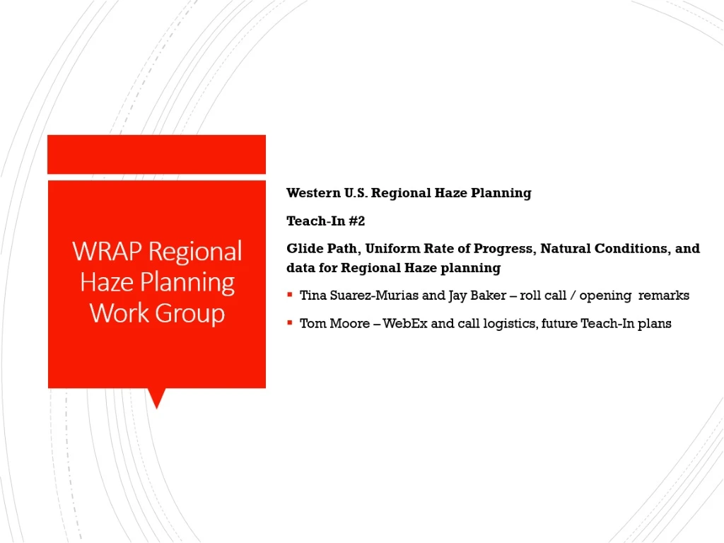
Review upcoming Teach-Ins and participation in WRAP Regional Haze Planning Work Group - Jay Baker and Tina Suarez-Murias
UNIFORM RATE OF PROGRESS ...AND THE GLIDE PATH – applying this conceptual planning approach From Here? 9-15-1982 WRAP Regional Haze Planning Work Group Regional Haze Teach-In #2 July 27, 2017 To There? 10-3-1982
Conceptual Planning Approach Clean Air Act Amendments of 1977 set National Goal: “…the prevention of any future, and the remedying of any existing impairment of visibility in mandatory class I Federal areas which impairment results from manmade air pollution.” Focus of 1999 Regional Haze Rule: Achieve Natural Conditions by 2064 • Construct a straight-line Glide Path using deciview units over time • Start point: Baseline Worst Visibility Averages for 2000-2004 • End Point: Worst Visibility under Natural Conditions,assigned to 2064 • Slope: the Uniform Rate of Progress • Prepare State SIP with Reasonable Progress Goals (RPGs) for each planning period • Do interim RPGs land on the Glide Path? • Why not? Worst Haze Days Baseline Uniform Rate of Progress (Slope of the Glide Path) RPG Worst Haze Days Average for Natural Conditions DECIVIEWS Best Days Baseline (must not be degraded) Additional time to reach Natural Conditions at initial rate Baseline (2000-2004) 2018 2064 YEAR
Moving from Concept to Reality CONCEPT: Assumptions for Achieving Natural Conditions at 2064 • Chemical species mass captured on IMPROVE filters, converted to deciviews, quantifies visibility • Natural Conditions are constant and expressed as deciview average for the worst haze days • All anthropogenic impacts can be eliminated, or reduced to be “not perceptible” at monitors • NCII deciview estimates assigned to 2064 can be refined by states with EPA approval REALITY: Both Natural Conditions and Causes of Haze are changing • Natural sources in West overwhelm anthropogenic reductions on haziest days • Using 2018 RPGs calculated through modeling, Western States set RPGs above the Glide Path • Public considers Glide Path the benchmark of progress and challenged RPGs and initial URPs • Progress is not straight line; 5-year deciview averages do not reflect anthropogenic emission trends • Western visibility improvements not discernible using deciview values alone • Current western visual range on average day is ~111 miles vs. ~58 miles at eastern IMPROVE monitors • Haze Algorithm was refined and estimates of Natural Conditions will change • Climate change, global economy, and political decisions affect natural sources Reality: Focus on reducing Controllable Anthropogenic Initial Concept: Eliminate Anthropogenic Impairment Uncontrollable Veneer Deciview Deciview Anthropogenic Haze (Representation of Alaskan site; each site has different mix of these three components) Natural Haze 5
Redefining Start and End Points of Glide Path • Baseline Years remain Start Point of Glide Path • Same baseline monitoring measurements, reinterpreted for second planning period • Species contributions initially related to emission sources by modeling were quantified • Natural Contributions determined mathematically using percentiles and substitution • Idealized Glide Path still Ends at 2064, but additional adjustments allowed • What will “Natural Conditions” actually be in the future? • Is the NCII or NCIII deciview level for the Worst Haze Days from Natural Sources only? • What deciview quantity actually comes from “uncontrollable sources”? • Should “known” baseline attributions be added to end point as surrogate placeholders? • Beyond 2064, will some of the uncontrollable U.S. anthropogenic emissions become controllable with future “as-yet-unknown” technologies? U.S. portion of this remaining uncontrollable veneer may or may not become controllable with future unknown technology?
Adjusted endpoint (adds components for International Emissions and Prescribed Burning to “Most Impaired Days” for Natural Conditions Glide Path Slope vs Uniform Rate of Progress 2018 RPG DECIVIEWS Adjust Baseline starting with Days “Most Impaired” by Anthropogenic Emissions by removing impacts from extreme natural episodic events Glide Path remains a straight-line benchmark for judging progress • Baseline (start point) and 2064 (endpoint) can change, so long-term slope changes • Baseline will be lower after adjustment to MID • 2064 endpoint will be higher after adjustment for “special accounting” emissions • Will 2064 endpoint change with better information incorporated each planning period? RPG and Uniform Rate of Progress determined for each planning period • Is progress in reducing impairment measured against the RPG or the Glide Path? Will need some outreach to explain changes to public expectations of progress... Initial Glide Path Best or Clearest Days Baseline (2000-2004) 2028 2064 2018 2038 2048 2058 YEAR Worst Natural Haze Days (WND) Most Anthropogenically Impacted Days (MID)
Focus on Anthropogenic Emissions 1. Define what is Anthropogenic and Controllable 2. Quantify all the emissions contributions on a daily basis for modelling Figure out relationship between source type and species light extinctions on a daily basis for modelling
Species’ Light Extinctions vs Source Contributions • Light Extinction Strength does not match relative mass emissions inventory • Per unit of mass: light extinction EC > OC > Nitrate > Sulfate > Fine Soil > Sea Salt > Coarse Mass • Species Extinction driving Highest Deciview Days in Western baselines different at each monitor • Mostly OC, Nitrates, Sulfates, and Coarse Mass • Some natural & some anthropogenic; international sources generate both • Baseline Composition is different on Most Anthropogenically Impaired Days (MIDs) • Expect Nitrates and Sulfates to dominate; perhaps some OC also • Future Natural Conditions (Worst Natural Haze Days) also estimated by Species Light Extinction • Expect Natural OC, Coarse Mass, and Fine Soil to be predominant in West • Is “NCII” (2064 endpoint) realistic? (circa 10 ug/m3 PM10 in top quintile of Worst Natural Haze Days!) • Is endpoint sum of highest quintile for natural sources of haze? • How should we quantify international and prescribed fire adjustments to “correct” Natural Conditions? • What about remaining uncontrollable U.S. anthropogenic emissions? 9.4 >>> 8.0 ug mass 31.3 >>> 7.8 ug mass Farthest Baseline Average Visibility 149 miles for All Days Shortest Baseline Average Visibility 93 miles for All Days
Challenges in Resetting Baseline • Species by species analysis time-consuming, but needed to select percentile • Compare every year of available data, bay annual average and by every day (for seasonality information) • Is 95th percentile correct for the specific site for specific species? • Or any site for any particular year? • Need protocol for daily substitution in days identified with e3 (above selected percentile) • Seasonal mean? Long-term average? 1x, 2x, 3x median for particular year? • Should every state use both OC+EC along with CM+FS • Will residential woodsmoke show up? • Will prescribed fire show up in wildfire percentile? • Will construction event show up in CM+FS record? • Will Hawaii be able to pinpoint volcanic emissions using percentile alone? • What to do with sites having <3 years of complete data? • Data substitution? Include 2005 or later? Understand site context and history, in addition to math! Relatively remote site, high elevation, longest data record in California shows change
Lassen Volcanic Case Study: 95th Percentile Compare seasonality with known fires and timing of prescribed burns. 2000 - no wildfires? 2001 - prescribed fires? 2002 - not all of Biscuit Fire? 2003 - maybe no wildfires 2004 - single day spike May 2004 If examined season by season, more likely that 15-30 Mm-1 could be prescribed fires, but over 30 Mm-1 is very likely associated with wildfire smoke – need consultation with Federal Land Managers for confirmation!
Possible Changes in Outcomes Worst Haze Days Light Extinction 2012 • Each monitor will have new MID baseline dv and long-term Glide Path to adjusted 2064 dv • Within each planning period, the interim URP slope will change • In theory, URP Slope based on 2014 MID dv start and 2028 MID dv forecast • Or, should we model for Worst Haze Days, adjust 2064, and use MID to measure progress? Initial Baseline Modeled 2018 RPG Extinction Potential corrections for MID
Modeling Challenge: Matching Reality All species unacceptably under-predicted for 2011 base year modeling at SEQU. How were baseline and NCIII calculated as start and finish of New Glide Path? Base year projections from 2011 – is West using 2014 as base year for 2028 forecast? Does 2028 forecast assume natural emissions are the same as 2011 (17-yr. span?)
Progress Report for 2018 Use Initial Glide Path and 2018 RPG calculation • Worst Haze Days Average for 2014-2018 (5-yr. avg.) • Compare with modeled 2018 RFP from initial RH SIP • Maintain consistency with WHD metric because modeling for 2018 RPGs attempted to account for uncontrollable factors • Top quintile includes natural & anthropogenic haze • Review benefits of BART controls after implementation • Verify emissions reductions of relevant precursors • Explain light extinction changes observed on Worst Days for species • Explain whether deciview reduction is discernible • Potential reasons for differences from modeled 2018 RPGs • Unexpected growth/decline of species in emissions forecast • Natural sources emissions different than predicted (e.g. baseline average held constant for wildfires) • Boundary Conditions changed due to global economy shifts or climate change • Confirm Best or Clearest Days from Baseline are maintained • Optional: Compare Visual Range on all days and publicize benefits Remember: the human eye detects haze at particle concentrations well below the NAAQS health standards!