Download
1 / 25
250 likes | 269 Views
Explore the CFSRL operational tables for radiosonde bias correction, highlighting the need for more continuous corrections, and the use of adaptive RAOB correction. Implement the R1 algorithm and Haimberger corrections for accurate data analysis.

E N D
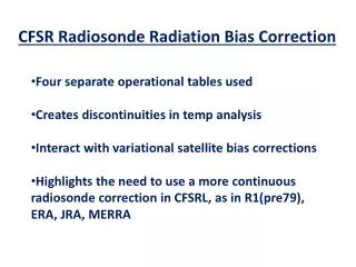
CFSR Radiosonde Radiation Bias Correction • Four separate operational tables used • Creates discontinuities in temp analysis • Interact with variational satellite bias corrections • Highlights the need to use a more continuous radiosonde correction in CFSRL, as in R1(pre79), ERA, JRA, MERRA
Plan for CFSRL adaptive RAOB correction • R1 used monthly F-O statistics to update radiosonde bias corrections by WMO block number before 1979 • So, port the R1 algorithm to CFSRL • Constrain the monthly corrections as documented in ERA40 which used a similar adaptive procedure • Also, look at the Haimberger corrections for the pre-satellite era. (83K+ days of corrections for a fixed set of individual stations) MERRA used modified R1 algorithm plus Haimberger corrections
Adaptive procedure devised for CFSRL Each month the composite (F-O) statistics for temperature are computed for each WMO block (01-99) A profile of percentages of the (F-O) stats is defined as follows: pob>=700 tfrac=0pob==500 tfrac=.8*.333pob==400 tfrac=.8*.666pob< 400 tfrac=.8A data density factor is defined: ddf=min(1,cnt/15)A limiting factor is defined: abs(cor)<=tfrac*2.5Next months corrections in each block is defined as: cor=(O-F)*tfrac*ddf. Finally the absolute value of the correction is limited to be <=tfrac*2.5.
Sample corrections in blocks 71-72 for Jul 2010 ---------------------------------------- ---------------------------------------- | 71 1.0 .0 .0 .0 .0 | 72 1.0 .0 .0 .0 .0 | | 71 2.0 .0 .0 .0 .0 | 72 2.0 .0 .0 .0 .0 | | 71 3.0 .0 .0 .0 .0 | 72 3.0 .0 .0 .0 .0 | | 71 5.0 1.0 .0 .8 .0 | 72 5.0 .0 .0 .1 .0 | | 71 7.0 -.5 .0 -.6 -.2 | 72 7.0 .0 .0 -.4 -.1 | | 71 10.0 -.9 .0 -.9 -.4 | 72 10.0 -.4 -.2 -.6 -.3 | | 71 20.0 -.2 .0 -.3 -.1 | 72 20.0 -.1 .1 -.2 -.3 | | 71 30.0 -.1 .0 -.1 -.3 | 72 30.0 .0 -.3 -.1 -.4 | | 71 50.0 .0 .0 -.1 .2 | 72 50.0 .0 .1 -.1 -.2 | | 71 70.0 -.1 .0 -.2 -.1 | 72 70.0 -.1 .4 -.1 -.3 | | 71 100.0 -.1 .0 -.1 -.1 | 72 100.0 .2 .2 .1 -.2 | | 71 150.0 .0 -.1 -.1 .0 | 72 150.0 .2 -.1 .2 .0 | | 71 200.0 .1 .0 .0 .3 | 72 200.0 .6 .2 .6 .4 | | 71 250.0 .4 .1 .3 .2 | 72 250.0 .4 -.1 .4 .2 | | 71 300.0 .2 .1 .2 .0 | 72 300.0 .2 -.1 .3 .1 | | 71 400.0 .1 -.1 .1 .0 | 72 400.0 .1 -.1 .1 .1 | | 71 500.0 .1 .0 .1 .0 | 72 500.0 .1 .0 .1 .1 | | 71 700.0 .0 .0 .0 .0 | 72 700.0 .0 .0 .0 .0 | | 71 850.0 .0 .0 .0 .0 | 72 850.0 .0 .0 .0 .0 | | 71 925.0 .0 .0 .0 .0 | 72 925.0 .0 .0 .0 .0 | | 71 1000.0 .0 .0 .0 .0 | 72 1000.0 .0 .0 .0 .0 | ---------------------------------------- ----------------------------------------