Download
1 / 107
1.3k likes | 1.76k Views
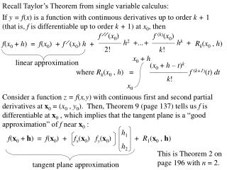
2. Economic Applications of Single-Variable Calculus. Derivative Origins Single Variable Derivatives Economic uses of Derivatives. 2. Economic Applications of Single-Variable Calculus. 2.1 Derivatives of Single-Variable Functions 2.2 Applications using Derivatives.

E N D
2. Economic Applications of Single-Variable Calculus • Derivative Origins • Single Variable Derivatives • Economic uses of Derivatives
2. Economic Applications of Single-Variable Calculus 2.1 Derivatives of Single-Variable Functions 2.2 Applications using Derivatives
2. Economic Applications of Single-Variable Calculus In economics, derivatives are used in various ways: • Marginal amounts (slope) • Maximization • Minimization • Sketching Graphs • Estimation
2.1 Derivatives of Single-Variable Functions Slope: -consider the following graph -the curved movement between A and B is approximated by the red straight line
2.1 – Quadratic example Slope Approximation: Slope = a decrease of 65 units over 4 time periods, or an average decrease of 16.25 A B
2.1 – Which is the slope at point B? Slope = rise/run =Δq/ Δp = (q1-q0)/(p1-p0) Slope AB =(q1-q0)/(p1-p0) =(35-100)/(3-1) =-65/2 =-32.5 Slope BC =(q1-q0)/(p1-p0) =(20-35)/(5-3) =-15/2 =-7.5 A B C
2.1 Derivatives of Single-Variable Functions -the slopes of these secants (AB and BC) reveal the rate of change of q in response to a change in p -these slopes change as you move along the curve -in order to find the slope AT B, one must use an INSTANTANEOUS SLOPE -slope of a tangent line
2.1 – Tangents A B C The green tangent line represents the instantaneous slope
2.1 Instantaneous Slope To calculate an instantaneous slope (using calculus), you need: • A function • A continuous function • A smooth continuous function
2.1.1 – A Function Definitions: -A function is any rule that assigns a maximum and minimum of one value to a range of another value -ie y=f(x) assigns one value (y) to each x -note that the same y can apply to many x’s, but each x has only one y -ie: y=x1/2 is not a function x = argument of the function (domain of function) f(x) or y = range of function
Function: y=0+2sin(2pi*x/14)+2cos(2pi*x/14) 4 3 2 1 0 x y -1 1 3 5 7 9 11 13 15 17 19 -2 -3 -4 x Each X Has 1 Y
Not a Function: Here each x Corresponds to 2 y values Often called the straight line test
2.1.1 – Continuous • -if a function f(x) draws close to one finite number L for all values of x as x draws closer to but does not equal a, we say: • lim f(x) = Lx-> a • A function is continuous iff (if and only iff) • f(x) exists at x=aii) Lim f(x) exists x->aiii) Lim f(x) = f(a) x->a
2.1.1 – Limits and Continuity • In other words: • The point must exist • Points before and after must exist • These points must all be joined • Or simply: • The graph can be drawn without lifting one’s pencil.
2.1.2 Smooth -in order for a derivative to exist, a function must be continuous and “smooth” (have only one tangent)
2.1.2 Derivatives • -if a derivative exists, it can be expressed in many different forms: • dy/dx • df(x)/dx • f ’(x) • Fx(x) • y’
2.1.2 Derivatives and Limits -a derivative (instantaneous slope) is derived using limits: This method is known as differentiation by first principles, and determines the slope between A and B as AB collapses to a point (A) B f(x+h) A f(x) h x+h x
2.1.2 Rules of Derivatives -although first principles always work, the following rules are more economical: 1) Constant Rule If f(x)=k (k is a constant),f ‘(x) = 0 2) General Rule If f(x) = ax+b (a and b are constants)f ‘ (x) = a
2.1.2 Examples of Derivatives 1) Constant Rule If f(x)=27 f ‘(x) = 0 2) General Rule If f(x) = 3x+12 f ‘(x) = 3
2.1.2 Rules of Derivatives 3) Power Rule If f(x) = kxn,f ‘(x) = nkxn-1 4) Addition Rule If f(x) = g(x) + h(x),f ‘(x) = g’(x) + h’(x)
2.1.2 Examples of Derivatives 3) Power Rule If f(x) = -9x7,f ‘(x) = 7(-9)x7-1 =-63x6 4) Addition Rule If f(x) = 32x -9x2f ‘(x) = 32-18x
2.1.2 Rules of Derivatives 5) Product Rule If f(x) =g(x)h(x),f ‘(x) = g’(x)h(x) + h’(x)g(x)-order doesn’t matter 6) Quotient Rule If f(x) =g(x)/h(x),f ‘(x) = {g’(x)h(x)-h’(x)g(x)}/{h(x)2}-order matters-derived from product rule (implicit derivative)
2.1.2 Rules of Derivatives 5) Product Rule If f(x) =(12x+6)x3f ‘(x) = 12x3 + (12x+6)3x2 = 48x3 + 18x26) Quotient Rule If f(x) =(12x+1)/x2f ‘(x) = {12x2 – (12x+1)2x}/x4= [-12x2-2x]/x4 = [-12x-2]/x3
2.1.2 Rules of Derivatives 7) Power Function Rule If f(x) = [g(x)]n,f ‘(x) = n[g(x)]n-1g’(x)-work from the outside in-special case of the chain rule 8) Chain Rule If f(x) = f(g(x)), let y=f(u) and u=g(x), thendy/dx = dy/du X du/dx
2.1.2 Rules of Derivatives 7) Power Function Rule If f(x) = [3x+12]4,f ‘(x) = 4[3x+12]33 = 12[3x+12]3 8) Chain Rule If f(x) = (6x2+2x)3 , let y=u3 and u=6x2+2x, dy/dx = dy/du X du/dx = 3u2(12x+2) = 3(6x2+2x)2(12x+2)
2.1.2 More Exciting Derivatives 1) Inverses If f(x) = 1/x= x-1,f ‘(x) = -x-2=-1/x2 1b) Inverses and the Chain Rule If f(x) = 1/g(x)= g(x)-1,f ‘(x) = -g(x)-2g’(x)=-1/g(x)2g’(x)
2.1.2 – More Exciting Derivatives 2) Natural Logs If y=ln(x), y’ = 1/x -chain rule may apply If y=ln(x2) y’ = (1/x2)2x = 2/x
2.1.2 – More Exciting Derivatives 3) Trig. Functions If y = sin (x), y’ = cos(x) If y = cos(x) y’ = -sin(x) -Use graphs as reminders
2.1.2 – More Derivatives Reminder: derivatives reflect slope:
2.1.2 – More Derivatives 3b) Trig. Functions – Chain Rule If y = sin2 (3x+2), y’= 2sin(3x+2)cos(3x+2)3 Exercises: y=ln(2sin(x) -2cos2(x-1/x)) y=sin3(3x+2)ln(4x-7/x3)5 y=ln([3x+4]sin(x)) / cos(12xln(x))
2.1.2 – More Derivatives 4) Exponents If y = bx y’ = bxln(b) Therefore If y = ex y’ = ex
2.1.2 – More Derivatives 4b) Exponents and chain rule If y = bkx y’ = bkxln(b)k Or more generally: If y = bg(x) y’ = bg(x)ln(b) X dg(x)/dx
2.1.2 – More Derivatives 4b) Exponents and chain rule If y = 52x y’ = 52xln(5)2 Or more complicated: If y = 5sin(x) y’ = 5sin(x)ln(5) * cos(x)
2.1.2.1 – Higher Order Derivatives -Until this point, we have concentrated on first order derivates (y’), which show us the slope of a graph -Higher-order derivates are also useful -Second order derivatives measure the instantaneous change in y’, or the slope of the slope -or the change in the slope:
2.1.2.1 Second Derivatives Here the slopeincreases as tincreases, transitioningfrom a negativeslope to a positiveslope. A second derivative would be positive, and confirm a minimum point on the graph.
2.1.2.1 Second Derivatives Here, the slope moves from positive to negative, decreasingover time. A second derivative would be negative and indicate a maximum point on the graph.
2.1.2.1 – Second Order Derivatives To take a second order derivative: • Apply derivative rules to a function • Apply derivative rules to the answer to (1) Second order differentiation can be shown a variety of ways: • d2y/dx2 b) d2f(x)/dx2 • f ’’(x) d) fxx(x) e) y’’
2.1.2.1 – Second Derivative Examples y=12x3+2x+11 y’=36x2+2 y’’=72x y=sin(x2) y’=cos(x2)2x y’’=-sin(x2)2x(2x)+cos(x2)2 y’’’=-cos(x2)2x(4x2)-sin(x2)8x-sin(x2)2x(2) =-cos(x2)8x3-sin(x2)12x
2.1.2.2 – Implicit Differentiation So far we’ve examined cases where our function is expressed: y=f(x) ie: y=7x+9x2-14 Yet often equations are expressed: 14=7x+9x2-y Which requires implicit differentiation. -In this case, y can be isolated. Often, this is not the case
2.1.2.2 – Implicit Differentiation Rules • Take the derivative of EACH term on both sides. • Differentiate y as you would x, except that every time you differentiate y, you obtain dy/dx (or y’) Ie: 14=7x+9x2-y d(14)/dx=d(7x)/dx+d(9x2)/dx-dy/dx 0 = 7 + 18x – y’ y’=7+18x
2.1.2.2 – Implicit Differentiation Examples Sometimes isolating y’ requires algebra: xy=15+x y+xy’=0+1 xy’=1-y y’=(1-y)/x (this can be simplified further) = [1-(15+x)/x]/x = (x-15-x)/x2 =(-15)/x2
2.1.2.2 – Implicit Differentiation Examples x2-2xy+y2=1 d(x2)/dx+d(2xy)/dx+d(y2)/dx=d1/dx 2x-2y-2xy’+2yy’=0 y’(2y-2x)=2y-2x y’=(2y-2x) / (2y-2x) y’=1
2.1.2.2 – Implicit Differentiation Examples Using the implicit form has advantages: 3x+7y8=18 3+56y7y’=0 56y7y’=-3 y’=-3/56y7 vrs. y=[(18-3x)/7)1/8 y’=1/8 * [(18-3x)/7)-7/8 * 1/7 * (-3) Which simplifies to the above.
2.2.1 Derivative Applications - Graphs Derivatives can be used to sketch functions: First Derivative: -First derivative indicates slope -if y’>0, function slopes upwards -if y’<0, function slopes downwards -if y’=0, function is horizontal -slope may change over time -doesn’t give shape of graph
2.2.1 Positive Slope Graphs Linear, Quadratic, and Lin-Log Graphs
2.2.1 Derivative Applications - Graphs Next, shape/concavity must be determined Second Derivative: -Second derivative indicates concavity -if y’’>0, slope is increasing (convex) -if y’’<0, slope is decreasing (concave, like a hill or a cave) -if y’’=0, slope is constant (or an inflection point occurs, see later)
2.2.1 Sample Graphs x’’= 2, slope is increasing; graph is convex
2.2.1 – Sample Graphs x’’=-2, slope is decreasing; graph is concave
2.2.1 Derivative Applications - Graphs Maxima/minima can aid in drawing graphs Maximum Point: If 1) f(a)’=0, and 2) f(a)’’<0, -graph has a maximum point (peak) at x=a Minimum Point: If 1) f(a)’=0, and 2) f(a)’’>0, -graph has a minimum point (valley) at x=a
2.2.1 Sample Graphs x’’= 2, slope is increasing; graph is convex x’=-10+2t=0t=5 Minimum