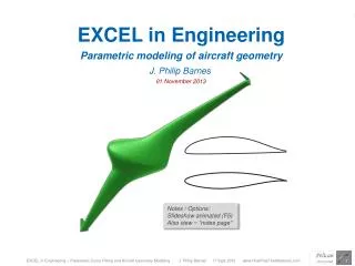
EXCEL in Engineering Parametric modeling of aircraft geometry

EXCEL in Engineering Parametric modeling of aircraft geometry J. Philip Barnes 01 November 2013 Notes / Options: Slideshow animated (F5) Also view ~ “notes page”

Presentation Contents • Getting started: EXCEL as a scientific spreadsheet • Misc., powerful Cartesian or parametric functions • Alternative iterative solution for x=f(x) • Linearize data before curve fit ~ “Pseudo-Gaussian” • Why go parametric? • High-order polynomial ~ theory & numerical method • De Casteljau-Bézier-Bernstein ~ history, review & renew • Parametric cubic spline~ theory & airfoil application • 3D visualization ~ concatenate maneuver rotations • Sneak preview: Rendering within EXCEL • Summary

Getting started: EXCEL as a scientific spreadsheet • Purpose (typical): • Read input and/or data from spreadsheet • Edit & run algorithm; generate new data • Write to spreadsheet cells & plot results • Copy all data & plots as new sheet; re-run • One-time setup: • EXCEL Options ~ Formulas ~ R1C1 ... • Trust Ctr. ~ settings ~ macro ~ enable & trust • Toolbar ~ more... ~ all ... ~ Visual Basic ~ Add • Set VB editor window to float on spreadsheet • Typical operations: • Type in the column headers, i.e. t, x, y, z • VB ~ insert ~ module ~ Type: sub example • Enter or edit code ~ save file as *.xlsm • Click “run” (note: module remains part of file) • Highlight applicable columns & plot the results • New case: Copy sheet, revise inputs, repeat 4)

Presentation Contents • Getting started: EXCEL as a scientific spreadsheet • Misc., powerful Cartesian or parametric functions • Alternative iterative solution for x=f(x) • Linearize data before curve fit ~ “Pseudo-Gaussian” • Why parametric? • High-order polynomial ~ theory & numerical method • De Casteljau-Bézier-Bernstein ~ history, review & renew • Parametric cubic spline~ theory & airfoil application • 3D visualization ~ concatenate maneuver rotations • Sneak preview: Rendering within EXCEL • Summary

Miscellaneous Geometry & curve-fit tools ~ Cartesian or parametric 1.0 1.0 Pseudo-Cosine 0.8 0.8 0.6 0.6 e = sin(hm p) 0.4 0.4 Pseudo-Sine 0.2 0.2 h 0.0 0.0 0.0 0.2 0.4 0.6 0.8 1.0 0.0 0.2 0.4 0.6 0.8 1.0 1.0 1.0 Exponential Varabola 0.8 0.8 e =e-5hm e = hm 0.6 0.6 0.4 0.4 0.2 0.2 h 0.0 0.0 0.0 0.2 0.4 0.6 0.8 1.0 0.0 0.2 0.4 0.6 0.8 1.0 0.5 m=1.0 2.0 m = 2.0 1.0 0.5 e y / ymax = cos m (hp/2) h x / xmax 0.5 m=1.0 2.0 EXCEL Exercise: Generate & plot 0.5 m=1.0 2.0

“Algebratross” math-modeled aircraft • Modeled entirely with Cartesian functions of earlier slide • Iterative solution for wing-body intersection (next topic)

Iterative solution for x = f(x) ~ stabilized and accelerated 0 < dy/dx < 1 dy/dx < 0 dy/dx > 1 y y y f(x) ' ALGORITHM, accel-stabilized iteration, x=f(x) ' guess = ... ' 1st guess ' i = 0 ' initialize iteration counter ' ,-> i = i + 1 ' increment iteration counter ' | if i = 1: x2 = guess ' 1st guess ' | if i = 2: x2 = 1.02 * guess ' 2nd guess ' | if i >= 3: ' | if dydx < 0: x2=(x1+y1)/2 ' half step ' | if 0<=dydx<=1: x2=2*y1 - x1 ' double step ' | if dydx > 1: x2=2*x1 - y1 ' reverse step ' | get y2 at x2 ' | test for exit criteria --> exit ' | if i >= 2 & x1#x2: dydx = (y2-y1)/(x2-x1) ' `- x1 = x2: y1 = y2 ' setup for next pass f(x) y=x • Basic: Guess x1 ; get y1 ; then set x2 = y1 • Refined: watch dy/dx ; modify "step" to (x2) • - Step mod aids convergence & stabilizes • Newton-Raphson may be faster or slower • Probability of convergence appears similar y=x y=x f(x) y1 y1 y1 x x x y1 y1 x2 x2 x1 y1 x2 x1 x1 Half step to accelerate: x2 = x1 - ½(x1-y1) = ½(x1+y1) Double step to accelerate: x2 = x1 - 2(x1-y1) = 2y1 - x1 Reverse step to stabilize: x2 = x1 +(x1-y1) =2x1-y1

Iterative solution for x = f(x) ~ example with six steps

“Pseudo-Gaussian” ~ First try to linearize ; then fit a polynomial y ≈ exp(-axb) Take ln twice: ln (-ln y) = ln a + b ln x y = a + b c polynomial? Apply (given x, get y): (1) cln x (2) y = f (c) ~ line or polynomial (3) y = exp (-exp y) • Physics are preserved • Meaningful extrapolation “Real life” data EXCEL Exercise: Fit polynom. y(c) Add 2 new columns Re-generate y(x)

Why go parametric? y EXCEL Exercise: Generate data (approx. this shape) t (0→1) ; tab & polynom. fit x(t), y(t) Plot x(t), y(t), y(x) t x • “Time” marches fwd; never encounter infinite rate • Let coordinates be parametric in “time” as x(t) & y(t) • Or, parametric with (q), as a circle x=rcosq ; y=rsinq • No problem with “wrap around” or curve crossing • Extend to 3 or more dimensions when applicable • Let all coordinates (x,y,z,w...) be parametric in (t) • Simply set (x = t) if (y, z, w) depend only on (x)

Polynomial ~ Parametric u(t) or Cartesian y(x) • Objective: Fit nth-order polynomial through (0_to_n) points • EXCEL is limited to (n=6) ; higher order is included herein • Use “0_to_n” VB arrays; shift the origin to the “0th point” • Then for coordinate u(t) with polynomial coefficients (c): • u-uo = c1(t-to) + c2(t-to)2 + ... ci(t-to)i ...+ cn(t-to)n • Shorthand: u = c1t + c2t2 + ... cit i ... + cntn • Matrix notation with polynomial applied at points 1 to n: u u ≡ u-uo n n 2 1 2 0 1 t t ≡ t-to • Solve linear system for coefficients (c); apply for, say, n=10:

Solution for 10th-order polynomial ~ Demo EXCEL Exercise: Experiment first by shifting one or more points, and second by increasing the order of the polynomial

Solution for 10th-order polynomial ~ Demo, right-to-left

De Casteljau-Bézier Curve ~ History,* Review & Renew • P. De Casteljaufirst conceived (1963) today’s “Bézier Curve” • His notes & algorithm remained proprietary at Citroën • Set (Np) Control points for control polygon near, not on, curve • (Np-1, Np-2,...) interpolation series on polygon-sides for x(t), y(t) • De Casteljau’s Algorithm is represented by the Bernstein Basis • as discovered by A.R. Forrest ~ Geometric construct → math • S. Bernstein’s polynomial (B) derivative (dB/dt) introduced herein • P. Bézier independently conceived (1966) the control polygon • Bézier’s algorithm is not used in today’s “Bezier Curve,” but • his work at Rénault was the foundation of UNISURF & CATIA p2 1/3 y p3 1/3 x,y 1/3 p1 pNp t = 1/3 x * R.T. Farouki, The Bernstein polynomial basis: a centennial retrospective, UC Davis, Mar 2012 * G. Farin, A History of Curves and Surfaces in CAGD, Arizona State University, 2007

De Casteljau Algorithm in action ~ close-up y p2 1/3 p3 t = 1/3 1/3 x,y 1/3 pNp p1 x Animated graphic (shift F5)

De Casteljau-Bézier-Bernstein (CBB) System in 2D ~ Demo x = S Bi Xpi p3 p4 N=Vxk V y = S Bi Ypi t p5 p2 p6 p1 V = (dx/dt) i + (dy/dt) j dx/dt = S (dB/dt)i Xpi dy/dt = S (dB/dt)i Ypi

Airfoil geometry modeling ~ “manual” C-B-B polygon pNp p1 p2 p3

Inverse solution for the De Casteljau-Bezier control polygon • Thus far we have “manually” set (Np) control-polygon points (P) • The C-B curve of (Nt) points approximates the desired trajectory • Solve for (P) so the C-B curve passes through(N) points (C) • Write C-B-B system with a square Bernstein Matrix (Np = Nt = N) • Approach: invert the Bernstein and Bernstein Rate Matrices • [C]=[B][P] ; [P]=[B]-1[C] ; [dC/dt]=[dB/dt][P] ; [P]=[dB/dt]-1 [dC/dt] For matrix inversion compact method & code, see: J.T. Golden, FORTRAN iV Programming and Computing, Prentice-Hall, 1965, p.114 p2 y p3 “time” t [B] usually not square c [B] & [B]-1 made square p1 cN pN c1 x

De Casteljau-Bezier-Bernstein Inverse Solution ~ First attempts 5-vertex circle 12-vertex airfoil pN-1 p2 pN p1 • Computed polygon (red) • BCC curve (black) • Specified points (white) Intent (via manual polygon) Result (via computed polygon) p3 c Polygon not shown t In each case, the computed polygon faithfully drove the curve through the specified points, but with unexpected side effects

Cubic spline ~ Parametric u(t) or Cartesian y(x) • Get smooth curve passing through (1_to_n) points • VB array dim. (n) elements: 0_to_n ~ ignore 0th elem. • 1st & 2nd derivative Continuity (3rd is not continuous) • Independently control L/R-end slope or 2nd derivative • Internal-node continuity yields tri-diagonal system • End constraints are applied in first and last rows • Parametric x(t) ; v  “velocity”; a  “acceleration” x n 3 2 1 t • Set ends; Solve linear EQs. for internal-knot accelerations (a)

Parametric cubic spline ~ Various end constraints “Stiff” ends “Flexible” ends “Flat” ends

Parametric cubic spline ~ Existing airfoil “fast & close match” L.E. radius T.E. slopes t “velocity” for tangent and normal vectors Fast, smooth & efficient design/characterization; 3 upper, 4 lower points; Add more points if req’d “velocity” for tangent and normal vectors

Laminar airfoil study ~ integrated geometric/aero design f Theodorsen Angle (f) • Velocity ratio Parametric cubic spline • Pressure coefficient Discontinuous 3rd-deriv. of cubic spline does not disrupt smooth airflow

Radius of curvature ~ Two coordinates parametric with “time” (t) y dy/dt v r dx/dt n x • Velocities & accelerations determine parametric curvature radius • Velocity is the tangent vector ; cross product yields normal vector • Application: Parametric-modeled airfoil leading-edge radius

“Trigonosoar” ~ 3D parametric model of aircraft geometry Chord, thickness, twist, etc. are parametric with spar coord. (p) from the centerline to winglet tip p ∫ds ≈S [(Dy)2 + (Dz)2 ] 0.5 z x y Aero axes

z z y x y c Aero axes Rotation Matrix Concatenation ~ Review and Renew • Define geometry only once • Apply maneuver transform Optionally include 90o rotation to translate from structural axes to aero axes

“Regenosoar” ~ math-modeled & visualized with tools herein

Rendering in EXCEL ~ using the "shapes" feature EXCEL Exercise: "Render" a circle with 5-pixel line thickness and red, green, & blue parametric with theta 1. Anchor optional background graphic top left at cell(1,1) 2. Generate object geometry (include normals & colors) 3. Render the object, pixel-by-pixel (via EXCEL "shapes")

Summary ~ EXCEL in Engineering / Geometry modeling y • EXCEL & VB provide capable scientific spreadsheet • Trigonometric functions ~ versatile & powerful • Suggestion: linearize data before fitting a curve • Iteration, x=f(x) ~ Alternative to Newton-Raphson • Parametric: multi-dimensions, wrap-around OK • De Casteljau-Bézier: labor-intense pass thru all pts. • Inverse Bézier runs thru all points ~ but with wild end effects • Polynomial passes thru all pts (no control at ends) • Polynomial advantages include simplicity & continuity • High-order polynomial can be quite robust • The cubic spline also passes through all points • With comprehensive control of start & end constraints • One application: efficiently design & characterize an airfoil • 3rd derivative not continuous, but geom. is “aero smooth” • EXCEL’s “shape” feature for graphics & rendering t x

About the Author Phil Barnes has a Bachelor’s Degree in Mechanical Engineering from the University of Arizona and a Master’s Degree in Aerospace Engineering from Cal Poly Pomona. He has 32-years of experience in performance analysis and computer modeling of aerospace vehicles, engines, and subsystems, primarily at Northrop Grumman. He has authored SAE technical papers on aerodynamics, dynamic soaring, and regenerative soaring. This latest presentation brings together Phil’s knowledge and passions for computer graphics, and geometry math modeling.

EXCEL in Engineering Parametric modeling of aircraft geometry

EXCEL in Engineering Parametric modeling of aircraft geometry

Presentation Transcript

PARAMETRIC SOLID MODELING AND DESIGN

Excel Financial Modeling

Financial Modeling in Excel

Modeling With Geometry

Parametric Modeling

Recent Parametric Instability Modeling

Modeling in Electrochemical Engineering

Introduction to Solid Modeling Parametric Modeling

Parametric Modeling

CPACS - Common Parametric Aircraft Configuration Schema

Excel – Engineering Statistics

aircraft engineering in india

2001 Citation Excel Aircraft

Real Estate Financial Modeling in Excel

A Comparison of Modeling Scales in Flexible Parametric Models

Solution of a System of ODEs with POLYMATH and Excel, Parametric Studies with Excel

Parametric Modeling

Sequential Calculations with POLYMATH and Excel, Parametric Studies with Excel

CPACS - Common Parametric Aircraft Configuration Schema

Introduction to Parametric Modeling

Spring Design using Parametric Modeling

financial modeling excel training