UNIT 3-Introduction-data mining

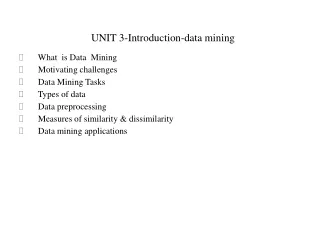
1. UNIT 3-Introduction-data mining • What is Data Mining • Motivating challenges • Data Mining Tasks • Types of data • Data preprocessing • Measures of similarity & dissimilarity • Data mining applications

2. Introduction-data mining • Many Definitions • Non-trivial extraction of implicit, previously unknown and potentially useful information from data • Exploration & analysis, by automatic or semi-automatic means, of large quantities of data in order to discover meaningful patterns

3. Data Mining Challenges • Scalability • Dimensionality • Complex and Heterogeneous Data • Data Quality • Data Ownership and Distribution • Privacy Preservation • Streaming Data

4. Data Mining Tasks • Prediction Methods • Use some variables to predict unknown or future values of other variables. • Description Methods • Find human-interpretable patterns that describe the data.

5. Data Mining Tasks • Classification [Predictive] • Clustering [Descriptive] • Association Rule Discovery [Descriptive] • Sequential Pattern Discovery [Descriptive] • Regression [Predictive] • Deviation Detection [Predictive]

6. Classification • Given a collection of records (training set ) • Each record contains a set of attributes, one of the attributes is the class. • Find a model for class attribute as a function of the values of other attributes. • Goal: previously unseen records should be assigned a class as accurately as possible. • A test set is used to determine the accuracy of the model. Usually, the given data set is divided into training and test sets, with training set used to build the model and test set used to validate it.

7. Classification -Example • Fraud Detection • Goal: Predict fraudulent cases in credit card transactions. • Approach: • Use credit card transactions and the information on its account-holder as attributes. • When does a customer buy, what does he buy, how often he pays on time, etc • Label past transactions as fraud or fair transactions. This forms the class attribute. • Learn a model for the class of the transactions. • Use this model to detect fraud by observing credit card transactions on an account.

8. Clustering-Definition • Given a set of data points, each having a set of attributes, and a similarity measure among them, find clusters such that • Data points in one cluster are more similar to one another. • Data points in separate clusters are less similar to one another. • Similarity Measures: • Euclidean Distance if attributes are continuous. • Other Problem-specific Measures.

9. Clustering-Example of an Application • Market Segmentation: • Goal: subdivide a market into distinct subsets of customers where any subset may conceivably be selected as a market target to be reached with a distinct marketing mix. • Approach: • Collect different attributes of customers based on their geographical and lifestyle related information. • Find clusters of similar customers. • Measure the clustering quality by observing buying patterns of customers in same cluster vs. those from different clusters.

10. Association Rule Discovery-definition • Given a set of records each of which contain some number of items from a given collection; • Produce dependency rules which will predict occurrence of an item based on occurrences of other items.

11. Association Rule Discovery: Application • Supermarket shelf management. • Goal: To identify items that are bought together by sufficiently many customers. • Approach: Process the point-of-sale data collected with barcode scanners to find dependencies among items. • A classic rule – • If a customer buys diaper and milk, then he is very likely to buy beer. • So, don’t be surprised if you find six-packs stacked next to diapers!

12. Sequential pattern discovery-definition • Given is a set of objects, with each object associated with its own timeline of events, find rules that predict strong sequential dependencies among different events. • Rules are formed by first discovering patterns. Event occurrences in the patterns are governed by timing constraints.

13. Example of Sequential pattern discovery • In telecommunications alarm logs, • (Inverter_Problem Excessive_Line_Current) • (Rectifier_Alarm) --> (Fire_Alarm) • In point-of-sale transaction sequences, • Computer Bookstore: • (Intro_To_Visual_C) (C++_Primer) --> (Perl_for_dummies,Tcl_Tk) • Athletic Apparel Store: • (Shoes) (Racket, Racketball) --> (Sports_Jacket)

14. Regression • Predict a value of a given continuous valued variable based on the values of other variables, assuming a linear or nonlinear model of dependency. • Greatly studied in statistics, neural network fields. • Examples: • Predicting sales amounts of new product based on advertising expenditure. • Predicting wind velocities as a function of temperature, humidity, air pressure, etc. • Time series prediction of stock market indices.

15. Deviation/Anomaly • Detect significant deviations from normal behavior • Applications: • Credit Card Fraud Detection • Network Intrusion Detection

16. Types of Data • Record • Data Matrix • Document Data • Transaction Data • Graph • World Wide Web • Molecular Structures • Ordered • Spatial Data • Temporal Data • Sequential Data • Genetic Sequence Data

17. Record Data . • Data that consists of a collection of records, each of which consists of a fixed set of attributes.

18. Data Matrix • If data objects have the same fixed set of numeric attributes, then the data objects can be thought of as points in a multi-dimensional space, where each dimension represents a distinct attribute • Such data set can be represented by an m by n matrix, where there are m rows, one for each object, and n columns, one for each attribute.

19. Document Data • Each document becomes a `term' vector, • each term is a component (attribute) of the vector, the value of each component is the number of times the corresponding term occurs in the document.

20. Transaction data • A special type of record data, where • each record (transaction) involves a set of items. • For example, consider a grocery store. The set of products purchased by a customer during one shopping trip constitute a transaction, while the individual products that were purchased are the items.

21. Graph Data • Examples: Generic graph and HTML Links

22. Ordered Data • Sequences of transactions

23. Data preprocessing • Aggregation • Sampling • Dimensionality Reduction • Feature subset selection • Feature creation • Discretization and Binarization • VariableTransformation

24. Aggregation • Combining two or more attributes (or objects) into a single attribute (or object) • Purpose • Data reduction - Reduce the number of attributes or objects • Change of scale - Cities aggregated into regions, states, countries, etc • More “stable” data - Aggregated data tends to have less variability

25. Aggregation • Variation of Precipitation in Australia Standard Deviation of Average Yearly Precipitation Standard Deviation of Average Monthly Precipitation

26. Sampling • Sampling is the main technique employed for data selection. • It is often used for both the preliminary investigation of the data and the final data analysis. • Statisticians sample because obtaining the entire set of data of interest is too expensive or time consuming. • Sampling is used in data mining because processing the entire set of data of interest is too expensive or time consuming. .

27. Types of Sampling • Simple Random Sampling • There is an equal probability of selecting any particular item • Sampling without replacement • As each item is selected, it is removed from the population • Sampling with replacement • Objects are not removed from the population as they are selected for the sample. • In sampling with replacement, the same object can be picked up more than once • Stratified sampling • Split the data into several partitions; then draw random samples from each partition

28. Dimensionality Reduction • Purpose: • Avoid curse of dimensionality • Reduce amount of time and memory required by data mining algorithms • Allow data to be more easily visualized • May help to eliminate irrelevant features or reduce noise • Techniques: • Principle Component Analysis • Singular Value Decomposition • Others: supervised and non-linear techniques

29. Dimensionality Reduction • PCA - Goal is to find a projection that captures the largest amount of variation in data. Mean is removed. Used in Pattern finding techniques. • SVD – Mean is not removed. Documents in newspaper can be associated with strongest components like game, play, lead, team, score, rebound, season, coach, league, goal with sports.

30. Feature Subset selection • Another way to reduce dimensionality of data • Redundant features • duplicate much or all of the information contained in one or more other attributes • Example: purchase price of a product and the amount of sales tax paid • Irrelevant features • contain no information that is useful for the data mining task at hand • Example: students' ID is often irrelevant to the task of predicting students' GPA

31. Feature subset selection • Techniques: • Brute-force approach: Try all possible feature subsets as input to data mining algorithm • Embedded approaches: Feature selection occurs naturally as part of the data mining algorithm • Filter approaches: Features are selected before data mining algorithm is run • Wrapper approaches: Use the data mining algorithm as a black box to find best subset of attributes

32. Feature Creation • Create new attributes that can capture the important information in a data set much more efficiently than the original attributes • Three general methodologies: • Feature Extraction • domain-specific • Mapping Data to New Space • Feature Construction • combining features

33. Discretization and Binarization • Discretization – It involves transforming continuous attribute into a categorical attribute • Binarization – It involves transforming both continuous and discrete attributes into one or more binary attributes

34. Variable Transformation • A function that maps the entire set of values of a given attribute to a new set of replacement values such that each old value can be identified with one of the new values • Simple functions: xk, log(x), ex, |x| • Standardization and Normalization

35. Measures of Similarity and Dissimilarity • Similarity • Numerical measure of how alike two data objects are. • Is higher when objects are more alike. • Often falls in the range [0,1] • Dissimilarity • Numerical measure of how different are two data objects • Lower when objects are more alike • Minimum dissimilarity is often 0 • Upper limit varies • Proximity refers to a similarity or dissimilarity

36. Euclidean Distance • Euclidean Distance • Where n is the number of dimensions (attributes) and pk and qk are, respectively, the kth attributes (components) or data objects p and q. • Standardization is necessary, if scales differ.

37. Minkowski Distance • Minkowski Distance is a generalization of Euclidean Distance Where r is a parameter, n is the number of dimensions (attributes) and pk and qk are, respectively, the kth attributes (components) or data objects p and q.

38. Common properties of a Distance • Distances, such as the Euclidean distance, have some well known properties. • d(p, q)  0 for all p and q and d(p, q) = 0 only if p= q. (Positive definiteness) • 2. d(p, q) = d(q, p) for all p and q. (Symmetry) • d(p, r)  d(p, q) + d(q, r) for all points p, q, and r. (Triangle Inequality) where d(p, q) is the distance (dissimilarity) between points (data objects), p and q. • A distance that satisfies these properties is a metric

39. Similarity between Binary Vectors • Common situation is that objects, p and q, have only binary attributes • Compute similarities using the following quantities M01 = the number of attributes where p was 0 and q was 1 M10 = the number of attributes where p was 1 and q was 0 M00 = the number of attributes where p was 0 and q was 0 M11 = the number of attributes where p was 1 and q was 1 • Simple Matching and Jaccard Coefficients SMC = number of matches / number of attributes = (M11 + M00) / (M01 + M10 + M11 + M00) J = number of 11 matches / number of not-both-zero attributes values = (M11) / (M01 + M10 + M11)

40. SMC versus Jaccard: Example Problem p = 1 0 0 0 0 0 0 0 0 0 q = 0 0 0 0 0 0 1 0 0 1 M01 = 2 (the number of attributes where p was 0 and q was 1) M10 = 1 (the number of attributes where p was 1 and q was 0) M00 = 7 (the number of attributes where p was 0 and q was 0) M11 = 0 (the number of attributes where p was 1 and q was 1) SMC = (M11 + M00)/(M01 + M10 + M11 + M00) = (0+7) / (2+1+0+7) = 0.7 J = (M11) / (M01 + M10 + M11) = 0 / (2 + 1 + 0) = 0

41. Cosine Similarity-Example problem • If d1 and d2 are two document vectors, then cos( d1, d2 ) = (d1d2) / ||d1|| ||d2|| , where  indicates vector dot product and || d || is the length of vector d. • Example: d1= 3 2 0 5 0 0 0 2 0 0 d2 = 1 0 0 0 0 0 0 1 0 2 d1d2= 3*1 + 2*0 + 0*0 + 5*0 + 0*0 + 0*0 + 0*0 + 2*1 + 0*0 + 0*2 = 5 ||d1|| = (3*3+2*2+0*0+5*5+0*0+0*0+0*0+2*2+0*0+0*0)0.5 = (42) 0.5 = 6.481. ||d2|| = (1*1+0*0+0*0+0*0+0*0+0*0+0*0+1*1+0*0+2*2)0.5= (6) 0.5 = 2.245 cos( d1, d2 ) = .3150

42. Data Mining Application 1. Prediction and description 2. Relationship marketing 3. Customer profiling 4. Outliers identification and detecting fraud 5. Customer segmentation 6. Website design and promotion.