5. Combination of random variables

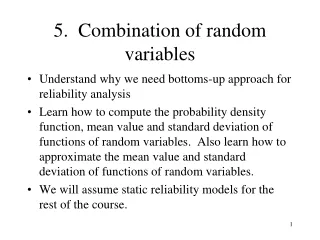
1. 5. Combination of random variables • Understand why we need bottoms-up approach for reliability analysis • Learn how to compute the probability density function, mean value and standard deviation of functions of random variables. Also learn how to approximate the mean value and standard deviation of functions of random variables. • We will assume static reliability models for the rest of the course.

2. Bottoms-up approach for reliability analysis Select primitive random variables Data and judgment Probability distributions of primitive random variables Relation between performance and primitive random variables Probability calculus Reliability or failure probability

3. Why bottoms-up approach for reliability analysis • Sometimes we do not have enough failure data to estimate reliability of a system. Examples: buildings, bridges, nuclear power plants, offshore platforms, ships • Solution: Bottom up approach for reliability assessment: start with the probability distributions of the primitive (generic random variables), derive probability distribution of performance variables (e.g. failure time). • Advantages: • Estimate probability distribution of input random variables (e.g., yield stress of steel, wind speed). Use the same probability distribution of the generic random variables in many different problems. • Identify and reduce important sources of uncertainty and variability.

4. Transformation of random variables • y=g(x) • Objective: given probability distribution of X, and function g(.), derive probability distribution of Y.

5. Transformation of random variables Y One-to-one transformation y=g(x) y+Dy y x x+Dx X

6. General transformationmultiple-valued inverse function

7. Functions of many variables Y2 X2 Ay Ax Y1 X1

8. Expectation (mean value) and variance • In many problems it is impractical to estimate probability density functions so we work with mean values (expectations) and variances • Expectation • E(aX)=aE(X) • E(X+Y)=E(X)+E(Y) • If X, Y independent, then E(XY)=E(X)E(Y)

9. Variance

10. Positive covariance Y X Covariance • Covariance measures the degree to which two variables tend to increase to decrease together Negative covariance Y X

11. Correlation coefficient • Correlation coefficient, : covariance normalized by the product of standard deviations • Ranges from –1 to +1 • Uncorrelated variables: correlation coefficient=0

12. Relation between correlation and statistical dependence • If X, Y independent then they are uncorrelated • If X, Y are uncorrelated, then they may be dependent or independent Uncorrelated variables Independent variables

13. Variance of uncorrelated variables

14. Chebyshev’s inequality • Upper bound of probability of a random variable deviating more than k standard deviations from its mean value • P(|Y-E(Y)|k)1/k2 • Upper bound is to large to be useful

16. Approximations for mean and variance of a function of random variables • Function of one variable: g(X) • E(g(X))=g(E(X)) • Standard deviation of g(X)=[dg(X)/dX]standard deviation of X • Derivative of g(X) is evaluated at the mean value of X

17. Approximations for mean and variance of a function of random variables • Function of many variables: g(X1,…,Xn) • E(g(X1,…,Xn))=g(E(X1),…, E(Xn)) • Variance of g(X) = [dg(X1,…,Xn)/dXi]2×variance of Xi+ 2 [dg(X1,…,Xn)/dXi]× [dg(X1,…,Xn)/dXj]×covariance of Xi,Xj • Derivatives of g(X) are evaluated at the mean value of X

18. When are the above approximations good? • When the standard deviations of the independent variables are small compared to their average values • Function g(X) is mildly nonlinear i.e. the derivatives do not change substantially when the independent variables change