Summary statistics
Summary statistics. Using a single value to summarize some characteristic of a dataset. For example, the arithmetic mean (or average) is a summary statistic because it gives the average value of a dataset such as average blood pressure readings. 4.1 Indices of Central Tendency (or location).

Summary statistics
E N D
Presentation Transcript
Summary statistics Using a single value to summarize some characteristic of a dataset. For example, the arithmetic mean (or average) is a summary statistic because it gives the average value of a dataset such as average blood pressure readings
4.1 Indices of Central Tendency (or location) (Arithmetic) Mean: average of a set of values Blood Pressure Readings Xi 95 X1 98 X2 101 X3 87 X4 105 X5 ---------------- 486 Sum Arithmetic Mean = = 486 / 5 = 97.2 mm Hg
4.2 Robust Measure of Location Mean is very sensitive (not robust) to extreme values Blood Pressure Readings Xi 87 X1 95 X2 98 X3 101 X4 1050 X5 87 95 98 101 105.0 Mean = 97.2 Decimal overlooked, Mean = 286.2
Robust measure of location The median (the middle value of an ordered data set) is less sensitive (robust) to extreme values in the data Blood Pressure Readings Xi 87 X1 95 X2 98 X3 101 X4 1050 X5 87 95 98 101 105 median value = 98 is unchanged Trimmed mean (e.g. 10% trimmed mean is the average after deleting 10% of the data at both ends) is also less affected by extreme values
Intervals between failures of an air conditioner (in operating hours) 413, 14, 58, 37, 100, 65, 9, 169, 447, 184, 36, 201, 118, 34, 31, 18, 19, 67, 57, 62, 7, 22, 34, 90, 10 Mean = ? 8% trimmed mean = ? Median = ?
Ordered values 7, 9, 10, 14, 18, 19, 22, 31, 34, 34, 36, 37, 57, 58, 62, 65, 67, 90, 100, 118, 169, 184, 201, 413, 447 Measures of location Sample size = 25 mean = 2302/25 = 92.1 hrs 8% of 25 = 2, leave out 2 obs at both ends 8% trimmed mean = 1426/21 = 67.9 hrs median = 13th ordered value = 57 < 67.9 <92.1 hrs
Desirable properties of the median • Not sensitive to extreme values in data • More suitable for describing skewed distributions (e.g., median income vs average income) • The relative positions of the data points are unchanged when log-transformed. As a result, the median of the log-transformed data is just the log of the median of the original data • Not so for the mean, the mean of logX is not obtainable from the mean of X 87 < 95 < 98 < 101 < 105 Med = 98
Relative positions of median and mean for skewed distributions Positively-skewed or skewed to the right (where the longer tail is) Mean > Median Negatively-skewed or skewed to the left (where the longer tail is) Mean < Median
When to use mean or median: Use both by all means. Mean performs best when we have a normal or symmetric distribution with thin tails. If skewed or when we want to limit the influence of outliers, use the median.
Indices of Dispersion or Spread Range: difference between the largest and the smallest value Problem: does not consider how values in between are scattered. In the following, for both sets of data, the numbers of observations, means, medians and ranges are all equal. Which one has more scatter? datasets with same range but different scatter of values 10, 12, 13, 14, 15, 16, 17, 18, 20 10, 15, 15, 15, 15, 15, 15, 15, 20 range
Indices of Dispersion A good index of dispersion should be one that summarises the dispersion of individual values from some central value like the mean mean X X X X X X
Indices of Dispersion Problem with averaging deviations of individual values from the mean is that it is always 0 87 - 97.2 = -10.2 95 - 97.2 = -2.2 98 - 97.2 = 0.8 101-97.2 = 3.8 105-97.2 = 7.8 --- 0 where 97.2 is the mean of values 87, 95, 98, 101, 105 average of deviations of individual values from the mean
Indices of Dispersion Usual approach: consider square deviations from the mean and take their average 87 - 97.2 = -10.2 95 - 97.2 = -2.2 98 - 97.2 = 0.8 101-97.2 = 3.8 105-97.2 = 7.8 --- 0 104.04 4.84 0.64 14.44 60.84 ---------- 184.80 sum of squares of deviations from the mean
Variance calculation from a sample:customary to divide by n-1 (default option in most software) rather than by n 104.04 4.84 0.64 14.44 60.84 ---------- 184.80 effective sample size - also called degrees of freedom = 184.8 / 4 = 46.2
Variance of a sample Can be shown mathematically:
Why subtract 1 ? • Results in a better estimator of the population variance • Acknowledge the fact that the population mean is unknown and has to be estimated by the sample mean (effective sample size decreased by 1 for every parameter estimated) • No need to subtract 1 if we calculate variance using deviations from the population mean
Variance of a sample • Problem with variance is its awkward unit of measurement as values have been squared • Problem overcome by taking square root of variance - revert back to original unit of measurement Square root of the variance gives thestandard deviation
Sample Standard Deviation The Sample Standard Deviation (S or SD)
4.4 Robust Measure of Dispersion • Variance is defined as the mean of the squared deviations and as such is even more nonrobust to extreme values than the mean (an extreme deviation becomes even more extreme after squaring) • A robust measure of dispersion is IQR/1.35 • where IQR = 3rd quartile – 1st quartile • = Inter-quartile range The reason for dividing IRQ by 1.35 is to make it compatible with the standard deviation when the underlying distribution is normal
Intervals between failures of an air conditioner (in operating hours) 413, 14, 58, 37, 100, 65, 9, 169, 447, 184, 36, 201, 118, 34, 31, 18, 19, 67, 57, 62, 7, 22, 34, 90, 10 Mean = ? 8% trimmed mean = ? Median = ? SD=? IQR/1.35 = ?
Ordered values 7, 9, 10, 14, 18, 19, 22, 31, 34, 34, 36, 37, 57, 58, 62, 65, 67, 90, 100, 118, 169, 184, 201, 413, 447 Measures of location Sample size = 25 mean = 2302/25 = 92.1 hrs 8% of 25 = 2, leave out 2 obs at both ends 8% trimmed mean = 1426/21 = 67.9 hrs median = 13th ordered value = 57 < 67.9 <92.1 hrs Measures of dispersion SD = 115.5 hrs 1st quartile = 7th ordered value = 22 hrs 3rd quartile = 19th ordered value = 100 hrs IQR/1.35 = 78/1.35 = 57.8 hrs
5-Number Summary of a data set • Min, • 1st quartile • Median • 3rd quartile, • Max Represent graphically by a box plot