Download
1 / 39
390 likes | 558 Views
Updated Algorithmic Modeling Proposal for SERDES Tx and Rx. Cadence, SiSoft DesignCon IBIS Summit Feb 1, 2007. Contributors. C. Kumar, Cadence Hemant Shah, Cadence Barry Katz, SiSoft Walter Katz, SiSoft Mike Steinberger, SiSoft Todd Westerhoff, SiSoft. Algorithmic. Modeling trends.

E N D
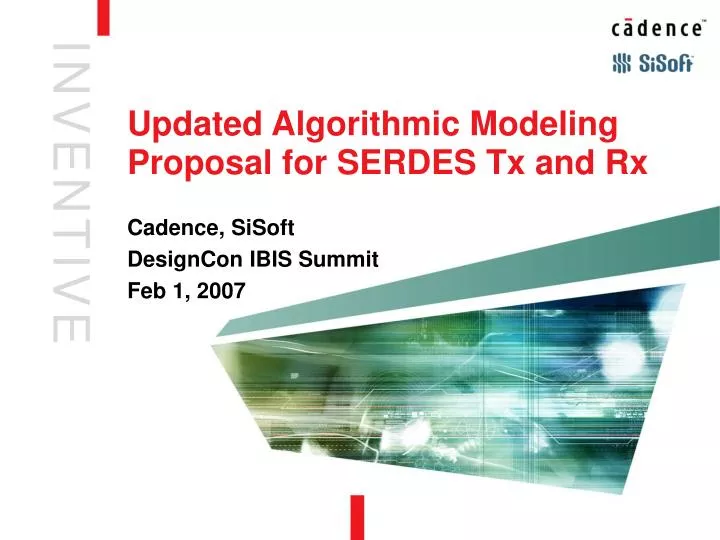
Updated Algorithmic Modeling Proposal for SERDES Tx and Rx Cadence, SiSoft DesignCon IBIS Summit Feb 1, 2007
Contributors • C. Kumar, Cadence • Hemant Shah, Cadence • Barry Katz, SiSoft • Walter Katz, SiSoft • Mike Steinberger, SiSoft • Todd Westerhoff, SiSoft
Algorithmic Modeling trends ‘98 ‘04 ‘05 IBIS Transistor Models • IBIS enjoyed 5 years as THE digital IO model format • Higher frequencies brought new issues and more skeptics • Gigabit serial links brought rapid transistor model increase in 2004 • Increasing Matlab use for algorithmic modeling • Lacks “interoperability”
Who Needs These Models? • System Designers • Predict end-end link BER and evaluate system-level design tradeoffs • ASIC designers • Evaluate different TX/RX architectures and behavior in hypothetical system environments • SerDes circuit designers • Validate with standard test beds • Measurement Equipment Vendors • Model device-specific equalization & clock recovery
High Speed Modeling – Then and Now • IBIS 1.0 – 1993 • Common clock design, ~25 MHz • Nonlinear drivers, uncontrolled impedances, reflections, ringing, irregular routing • Needed way to efficiently encapsulate push-pull output driver behavior • IBIS-ATM – 2007 • Serial link design, 3+ Gbps • Highly linear drivers, controlled transmission paths • Linear Time Invariant (LTI) network theory applies • Need way to model transmitter / receiver equalization, clock recovery behavior, predict BER
SerDes Proposal Discussion History • June 2006 – Initial Cadence proposal for SerDes device modeling • Sep 2006 – Arpad’s peak distortion analysis with VHDL-AMS • Oct 2006 – Cadence proposal in IBIS BIRD format • Based on request from the IBIS-ATM team • Dec 2006 - SiSoft proposes LTI modeling terminology • Today we share improvements to the original Cadence proposal • This team believes all major issues for the proposal in June / July by Cadence, IBM are addressed • Provides for future extensibility • Provides IBIS a unique opportunity take a leadership position in SerDes device modeling
Issues with Original Proposal • Network representation • Issue: concerns over whether impulse response compromised accuracy and pole/zero representation was required • Recommendation: Any time-domain or frequency-domain representation can be converted into any other. It’s true the impulse response must be long enough to contain needed low-frequency components, but this is readily achievable
Issues with Original Proposal • Model parameter representation • Issue: All parameters were IP vendor definable with no commonality; EDA tools need models to expose parameters in a standard way to consume them • Recommendation: addressed in this proposal • Methodology dependency • Issue: concern that “getwave” was predicated on a certain approach to time-domain convolution • Recommendation: addressed in this proposal
Analysis can be performed in either time or frequency domain Circuit behavior is “characterized” in terms of impulse response (time domain) or transfer function (frequency domain) This isn’t “circuit simulation” as much as “signal processing” Terminology and techniques may be new to digital designers, but methods are very well established (~40 years old) Let’s Talk LTI …
HSpice/Linear Modeling Correlation Studies http://www.vhdl.org/pub/ibis/summits/dec05/wang.pdf http://www.vhdl.org/pub/ibis/summits/jun05/huq.pdf
LTI Terminology • We’ll use definitions fromhttp://www.vhdl.org/pub/ibis/macromodel_wip/archive/20061212/toddwesterhoff/Serial%20Link%20Terminology/serial_link_terminology.pdf
The LTI Analysis Continuum Channel Impulse Response hTX(t) h(t) hRX(t) Channel Pulse Response (No EQ) p(t) hTX(t) h(t) hRX(t) Channel Pulse Response (TX EQ) hTE(t) p(t) hTX(t) h(t) hRX(t) Channel Pulse Response (TX, RX EQ) hRE(t) hTE(t) p(t) hTX(t) h(t) hRX(t) Equalized RX Data b(t) hRE(t) hTE(t) p(t) hTX(t) h(t) hRX(t) Billions of bits in a reasonable time Limited No
The LTI Analysis Continuum Channel Impulse Response hTX(t) h(t) hRX(t) Channel Pulse Response (No EQ) p(t) hTX(t) h(t) hRX(t) Channel Pulse Response (TX EQ) hTE(t) p(t) hTX(t) h(t) hRX(t) Channel Pulse Response (TX, RX EQ) hRE(t) hTE(t) p(t) hTX(t) h(t) hRX(t) Equalized RX Data b(t) hRE(t) hTE(t) p(t) hTX(t) h(t) hRX(t) Billions of bits in a reasonable time No
The LTI Analysis Continuum Channel Impulse Response hTX(t) h(t) hRX(t) Channel Pulse Response (No EQ) p(t) hTX(t) h(t) hRX(t) Channel Pulse Response (TX EQ) hTE(t) p(t) hTX(t) h(t) hRX(t) Channel Pulse Response (TX, RX EQ) hRE(t) hTE(t) p(t) hTX(t) h(t) hRX(t) Equalized RX Data b(t) hRE(t) hTE(t) p(t) hTX(t) h(t) hRX(t) Billions of bits in a reasonable time
The LTI Analysis Continuum Channel Impulse Response hTX(t) h(t) hRX(t) Channel Pulse Response (No EQ) p(t) hTX(t) h(t) hRX(t) Channel Pulse Response (TX EQ) hTE(t) p(t) hTX(t) h(t) hRX(t) Channel Pulse Response (TX, RX EQ) hRE(t) hTE(t) p(t) hTX(t) h(t) hRX(t) Equalized RX Data b(t) hRE(t) hTE(t) p(t) hTX(t) h(t) hRX(t) Billions of bits in a reasonable time
The LTI Analysis Continuum Channel Impulse Response hTX(t) h(t) hRX(t) Channel Pulse Response (No EQ) p(t) hTX(t) h(t) hRX(t) Channel Pulse Response (TX EQ) hTE(t) p(t) hTX(t) h(t) hRX(t) Channel Pulse Response (TX, RX EQ) hRE(t) hTE(t) p(t) hTX(t) h(t) hRX(t) Equalized RX Data b(t) hRE(t) hTE(t) p(t) hTX(t) h(t) hRX(t) Billions of bits in a reasonable time
The LTI Analysis Continuum Channel Impulse Response hTX(t) h(t) hRX(t) Channel Pulse Response (No EQ) p(t) hTX(t) h(t) hRX(t) Channel Pulse Response (TX EQ) hTE(t) p(t) hTX(t) h(t) hRX(t) Channel Pulse Response (TX, RX EQ) hRE(t) hTE(t) p(t) hTX(t) h(t) hRX(t) Equalized RX Data b(t) hRE(t) hTE(t) p(t) hTX(t) h(t) hRX(t) Billions of bits in a reasonable time
The LTI Analysis Continuum Channel Impulse Response hTX(t) h(t) hRX(t) Channel Pulse Response (No EQ) p(t) hTX(t) h(t) hRX(t) Channel Pulse Response (TX EQ) hTE(t) p(t) hTX(t) h(t) hRX(t) Channel Pulse Response (TX, RX EQ) hRE(t) hTE(t) p(t) hTX(t) h(t) hRX(t) Equalized RX Data b(t) hRE(t) hTE(t) p(t) hTX(t) h(t) hRX(t) Billions of bits in a reasonable time
Defining a Standard • Serial channel analysis involves a combination of circuit simulation and signal processing techniques • There are many ways to combine the two sets of analyses • A meaningful standard must define explicitly what data the models consume and produce • It’s useful to show how the models can be employed in the context of a specific analysis process • The example process doesn’t mean this is the only way the models can be used
Two Main Analysis Schemes • Impulse Response Processing (“Init”) • Channel impulse response is obtained from circuit analysis • Transmitter equalization is applied • Receiver equalization is applied • Recovered clock behavior is predicted • Waveform Processing (“GetWave” – bit by bit sim) • Time-Domain waveform can come from any simulation method • Transmit equalization is applied • Receive equalization is applied • Recovered clock behavior is predicted
Obtaining The Equalized Impulse Response Control Settings Control Settings • Channel impulse is passed to transmitter model, model returns impulse after transmit equalization • Resulting impulse is passed to receiver model, model returns impulse after receive equalization, along with recovered clock distribution Transmitter AlgorithmicModel Receiver AlgorithmicModel With TX, RX EQ With TX EQ Channel Impulse Response Clock Distribution
Transmitter Algorithmic Model Updated (Filtered)Impulse Response V(t) Impulse Response V(t) Standard Device Settings OptimizedDevice Settings (Optional) Model-Specific Device Settings (Optional)
Receiver Algorithmic Model - Init Updated (Filtered)Impulse Response V(t) Impulse Response V(t) Recovered ClockDistribution Standard Device Settings OptimizedDevice Settings (Optional) Model-Specific Device Settings (Optional)
ReceiveEqualization Transmitter ElectricalCharacteristics Receiver ElectricalCharacteristics TransmitEqualization ChannelCharacteristics Equalized Impulse Response ChannelImpulse Response Signal Processing Circuit Simulation Equalized Impulse Response Processing hTX(t) h(t) hRX(t) hTE(t) hRE(t)
Receiver Algorithmic Model - GetWave Updated (Filtered)Waveform Stream V(t) Waveform stream V(t) Recovered ClockDistribution Standard Device Settings OptimizedDevice Settings (Optional) Model-Specific Device Settings (Optional)
Algorithmic Models • Need defined standard for input and output time-domain waveform formats • Need standard defined parameters, indicating which parameters are required (if any) • Need a standard mechanism for defining additional model-specific parameters • Can be implemented in any language or scheme that allows them to accept input and produce output as defined (black box)
S Equalizer Sampler Clock Recovery IBIS Support for Algorithmic Modeling [Component] MY_COMP … [Model] ModelName Model_Type SerDes_TX • Existing IBIS buffer syntax • [Algorithmic Model] … • [End Algorithmic Model] Circuit Simulation Signal Processing
IBIS Algorithmic Modeling Extensions • Delimited with • [Algorithmic Model] … [End Algorithmic Model] • Reserved keywords for standard model parameters • Defined as part of IBIS standard, enables EDA “built-in” models • IP vendors can add keywords • [User-Defined Parameters] • Protects IP by using “black box” model to hide details of filtering and clock recovery/optimization algorithms
Defining Algorithmic Parameter Types & Syntax <keyword name> <usage> <data type> <data format> <values> <usage> In Parameter is required Input to executable Out Parameter is Output only from executable IO Optional Input to executable If input then its value will be used If output then its value will be determined by executable and will be in the output file (Note: Input parameters may be echoed into the executable output file) <data type> (default is float) float integer string <data format> (default to range) range <typ value> <min value> <max value> list <typ value> <value> <value> <value> ... <value> corner <typ value> <slow value> <fast value> table #columns Gaussian <mean> <sigma> Dual-Dirac <mean> <mean> <sigma> | Composite of two Gaussian DjRj <minDj> <maxDj> <sigma> | Convolve Gaussian (sigma) with uniform Modulation PDF
[IBIS Ver] 4.2 [File name] serdes_device.ibs [Date] 01/27/2007 [File Rev] 1.0 [Source] From HSpice and Matlab analysis | [Notes] Rev 1.0: 01/27/2007 - Initial model | [Component] MY_SERDES [Manufacturer] SERDESCORP [Package] |variable typ min max R_pkg 100m 50m 150m L_pkg 2.0nH 1.5nH 2.5nH C_pkg 0.8pF 0.6pF 1.0pF | | [Pin] signal_name model_name R_pin L_pin C_pin | A1 TX_ MY_TX A2 TX+ MY_TX B1 RX_ MY_RX B2 RX+ MY_RX |****************DIFF PIN****************** [Diff_pin] inv_pin vdiff tdelay_typ tdelay_min tdelay_max | A1 A2 NA 0ns NA NA B1 B2 .1V 0ps NA NA Sample IBIS Model
[Algorithmic Model] | | Executable (optional) Executable Solaris SerDesTx61.solaris Executable Linux SerDesTx61.linux Executable Windows SerDesTx61.windows | | TX Jitter Rj, Dj | Default to None Jitter DjRj 0 3ps 2ps | | Modulation Modulation NRZ | Default to NRZ | | Tap Data Taps 4 | Default to 4 Primary_Tap 2 | Default to 2 Tap_Gain_Min -1. -1. -1. -.25 | Default to -1. -1. -1. -1. Tap_Gain_Max 1. 1. 1. .25 | Default to 1. 1. 1. 1. Tap_Gain_Steps 32 32 32 8 | Default to infinite granularity Max_Tap_Sum 1. | Default 1. | | Tap Spacing | Default Synch Tap_Spacing Synch | Synch ' Bit_Time | Tap_Spacing 160p | Uniform spacing, but not bit_time | Tap_Spacing 160p 130p 120p | Non uniform spacing | [User Defined Parameters] | For executable only Secretsauce in integer range 5 1 9 [End User Defined Parameters] [End Algorithmic Model] | End Model MY_TX Sample IBIS Model - SerDes_TX | ********************************* | SERDES TRANSMITTER MODEL | ********************************* [Model] MY_TX Model_type SerDes_TX | Vmeas = 0.500V Vref = 0.500V Cref = 0.000F Rref = 50.000Ohm | typ min max | C_comp 1.00pF 0.80pF 1.20pF | [Voltage Range] 1.00V 0.95V 1.05V [Temperature Range] 60.0 100.0 0.0 | |*************************************************************************** | [Pulldown] | Voltage I(typ) I(min) I(max) ... [Pullup] | Voltage I(typ) I(min) I(max) ... |*************************************************************************** [Ramp] R_load = 50.00Ohm | typ min max dV/dt_r 781.447mV/372.457ps 737.729mV/382.334ps 823.953mV/385.013ps dV/dt_f 784.341mV/360.004ps 741.357mV/350.697ps 829.867mV/356.268ps | [Falling Waveform] V_fixture = 1.000V V_fixture_min = 0.95V V_fixture_max = 1.05V R_fixture = 50.00Ohm | | Time V(typ) V(min) V(max) | ...
[Algorithmic Model] | | Rx Optimize/Filter/ClockPDF Executable | Executable Models (Required) Executable Solaris SerDesRx61.solaris Executable Linux SerDesRx61.linux Executable Windows SerDesRx61.windows | | Reserved Parameter Names, Allowed Values Number_Aggressors integer range 0 0 8 | Default to 0 0 8 Modulation NRZ | Default to NRX Encoding string list scrambled 8b10b 64b66b | Default to scrambled Frequency_Offset 200u 0 600u | Default to 200u (200ppm Differential_Offset 10mV | Default to 10mV Decision Point Threshold Quality | Output by model if present (Bigger is Better) Taps 4 | Default to 4 Tap_Usage IO Primary_Tap 2 | Default to 2 Tap_Gain_Min -1. -1. -1. -.25 | Default to -1 -1 -1 -1 Tap_Gain_Max 1. 1. 1. .25 | Default to 1 1 1 1 Tap_Steps 64 64 64 16 | Default to infinite granularity Max_Tap_Sum 1. | Default to 1. Tap_Spacing Synch | Default to Synch=Bit_Time | clock_PDF table 2 | Optional If not returned by exe and if not | specified EDA tool will assume some default PDF -40ps 0 -30ps 1e-8 … 40ps 1e-8 50ps 0 end_table | [User Defined Parameters] Secretsauce IO integer range 5 1 9 BER | Output by model if present [End User Defined Parameters] [End Algorithmic Model] | End Model MY_RX [END] | ********************************* | SERDES RECEIVER MODEL | ********************************* | [Model] MY_RX Model_type SerDes_RX C_comp 1.00p 0.95p 1.05p | Vinl = 0.4 Vinh = 0.6 | [Temperature Range] 60 100 0 [Voltage Range] 1.0 0.95 1.05 [GND Clamp] ... [Power Clamp] ... Sample IBIS Model - SerDes_RX
Executing the Transmit Model SerDesTx61.solaris <Input file> <Output File> Output File Tap_Gain –2 26 -2 1 Strength .875 Frammistat 8 [Begin Impulse Response] ... [End Impulse Response] Input File Bit_Time 160ps Time_Step 10ps Strength 1. Frammistat 7 Tap_Gain –3 24 -3 1 [Begin Impulse Response] ... [End Impulse Response]
Executing the Receiver Model SerDesRx61.solaris <Input file> <Output File> Input File Bit_Time 160ps Time_Step 10ps Encoding 64b66b Frequency_Offset 200u Number_Aggressors 0 Frammistat 7 [Begin Impulse Response] 0. .01 .1 1 .1 .01 -.01 .01 [End Impulse Response] Output File Frammistat 9 [Begin Impulse Response] 0. .01 -.01 .01 [End Impulse Response] [Begin Clock PDF] … [End Clock PDF]
Executing the Receiver Model (“GetWave”) SerDesRx61.dll Input TD Waveform, Waveform Size Output Modified waveform Clock tics • AMI interface simplified based on feedback • Sample interval dropped, since it is set in the init call
Init .exe Tx .dll Rx Init .exe .dll .dll GetWave Executable Model Options
Summary • Serial link analysis involves two different types of simulation • Circuit simulation – for derivation of impulse response • LTI analysis – transmit/receive equalization and clock recovery • Existing IBIS models largely address circuit simulation needs • Equalization and clock recovery algorithms can be effectively modeled with IP vendor-supplied routines • Model calling sequence can be clearly defined and is user-extensible • This amended proposal addresses major issues discussed in IBIS-ATM meetings for the past 6 months • Leverages existing IBIS model parameters and circuit simulation infrastructure • Provides IP vendors ability to do as much as they wish in the (black box) model
Next Steps • Update BIRD • With documentation • Present to ATM (Target: Mid-February) • Detailed technical review • Present to IBIS Open Forum


![[SERDES Interface Block diagram]](https://cdn1.slideserve.com/3175187/slide1-dt.jpg)