Download
1 / 18
180 likes | 220 Views
This lecture covers topics such as branch prediction, out-of-order execution, and cache basics. It includes details about bimodal predictor table, memory hierarchy, and cache hierarchies.

E N D
Lecture 20: OOO, Memory Hierarchy • Today’s topics: • Branch prediction wrap-up • Out-of-order execution • Cache basics
Bimodal Predictor Table of 16K entries of 2-bit saturating counters 14 bits Branch PC Indexing functions Multiple branch predictors History, trade-offs
2-Bit Prediction • For each branch, maintain a 2-bit saturating counter: if the branch is taken: counter = min(3,counter+1) if the branch is not taken: counter = max(0,counter-1) … sound familiar? • If (counter >= 2), predict taken, else predict not taken • The counter attempts to capture the common case for each branch
Slowdowns from Stalls • Perfect pipelining with no hazards an instruction completes every cycle (total cycles ~ num instructions) speedup = increase in clock speed = num pipeline stages • With hazards and stalls, some cycles (= stall time) go by during which no instruction completes, and then the stalled instruction completes • Total cycles = number of instructions + stall cycles
Multicycle Instructions • Multiple parallel pipelines – each pipeline can have a different number of stages • Instructions can now complete out of order – must make sure that writes to a register happen in the correct order
An Out-of-Order Processor Implementation Reorder Buffer (ROB) Branch prediction and instr fetch Instr 1 Instr 2 Instr 3 Instr 4 Instr 5 Instr 6 T1 T2 T3 T4 T5 T6 Register File R1-R32 R1 R1+R2 R2 R1+R3 BEQZ R2 R3 R1+R2 R1 R3+R2 Decode & Rename T1 R1+R2 T2 T1+R3 BEQZ T2 T4 T1+T2 T5 T4+T2 ALU ALU ALU Instr Fetch Queue Results written to ROB and tags broadcast to IQ Issue Queue (IQ)
Example Code Completion times with in-order with ooo ADD R1, R2, R3 5 5 ADD R4, R1, R2 6 6 LW R5, 8(R4) 7 7 ADD R7, R6, R5 9 9 ADD R8, R7, R5 10 10 LW R9, 16(R4) 11 7 ADD R10, R6, R9 13 9 ADD R11, R10, R9 14 10
Cache Hierarchies • Data and instructions are stored on DRAM chips – DRAM is a technology that has high bit density, but relatively poor latency – an access to data in memory can take as many as 300 cycles today! • Hence, some data is stored on the processor in a structure called the cache – caches employ SRAM technology, which is faster, but has lower bit density • Internet browsers also cache web pages – same concept
Memory Hierarchy • As you go further, capacity and latency increase Disk 80 GB 10M cycles Memory 1GB 300 cycles L2 cache 2MB 15 cycles L1 data or instruction Cache 32KB 2 cycles Registers 1KB 1 cycle
Locality • Why do caches work? • Temporal locality: if you used some data recently, you will likely use it again • Spatial locality: if you used some data recently, you will likely access its neighbors • No hierarchy: average access time for data = 300 cycles • 32KB 1-cycle L1 cache that has a hit rate of 95%: average access time = 0.95 x 1 + 0.05 x (301) = 16 cycles
Accessing the Cache Byte address 101000 Offset 8-byte words 8 words: 3 index bits Direct-mapped cache: each address maps to a unique location in cache Sets Data array
The Tag Array Byte address 101000 Tag 8-byte words Compare Direct-mapped cache: each address maps to a unique address Tag array Data array
Example Access Pattern Byte address Assume that addresses are 8 bits long How many of the following address requests are hits/misses? 4, 7, 10, 13, 16, 68, 73, 78, 83, 88, 4, 7, 10… 101000 Tag 8-byte words Compare Direct-mapped cache: each address maps to a unique address Tag array Data array
Increasing Line Size Byte address A large cache line size smaller tag array, fewer misses because of spatial locality 10100000 32-byte cache line size or block size Tag Offset Tag array Data array
Associativity Byte address Set associativity fewer conflicts; wasted power because multiple data and tags are read 10100000 Tag Way-1 Way-2 Tag array Data array Compare
Associativity How many offset/index/tag bits if the cache has 64 sets, each set has 64 bytes, 4 ways Byte address 10100000 Tag Way-1 Way-2 Tag array Data array Compare
Example • 32 KB 4-way set-associative data cache array with 32 byte line sizes • How many sets? • How many index bits, offset bits, tag bits? • How large is the tag array?
Title • Bullet