Download
1 / 148
1.48k likes | 1.51k Views
VIII. Factorial designs at two levels. VIII.A Replicated 2 k experiments VIII.B Economy in experimentation VIII.C Confounding in factorial experiments VIII.D Fractional factorial designs at two levels. Factorial designs at two levels.

E N D
VIII. Factorial designs at two levels VIII.A Replicated 2k experiments VIII.B Economy in experimentation VIII.C Confounding in factorial experiments VIII.D Fractional factorial designs at two levels Statistical Modelling Chapter VIII
Factorial designs at two levels • Definition VIII.1: An experiment that involves k factors all at 2 levels is called a 2k experiment. • These designs represent an important class of designs for the following reasons: • They require relatively few runs per factor studied, and although they are unable to explore fully a wide region of the factor space, they can indicate trends and so determine a promising direction for further experimentation. • They can be suitably augmented to enable a more thorough local exploration. • They can be easily modified to form fractional designs in which only some of the treatment combinations are observed. • Their analysis and interpretation is relatively straightforward, compared to the general factorial. Statistical Modelling Chapter VIII
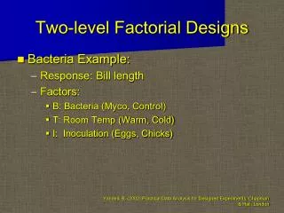
VIII.A Replicated 2k experiments • An experiment involving three factors — a 23 experiment — will be used to illustrate. a) Design of replicated 2k experiments, including R expressions • The design of this type of experiment is same as general case outlined in VII.A, Design of factorial experiments. • However, the levels used for the factors are specific to these two-level experiments. Statistical Modelling Chapter VIII
Notations for treatment combinations • Definition VIII.2: There are three systems of specifying treatment combinations in common usage: • Use a - for the low level of a quantitative factor and a + for the high level. Qualitative factors are coded arbitrarily but consistently as minus and plus. • Denote the upper level of a factor by a lower case letter used for that factor and the lower level by the absence of this letter. • Use 0 and 1 in place of - and +. • We shall use the notation as it relates to the computations for the designs. Statistical Modelling Chapter VIII
Example VIII.1 23 pilot plant experiment • An experimenter conducted a 23 experiment in which there are • two quantitative factors — temperature and concentration — and • a single qualitative factor — catalyst. • Altogether 16 tests were conducted with the three factors assigned at random so that each occurred just twice. • At each test the chemical yield was measured and the data is shown in the following table: Table also gives treatment combinations, using the 3 systems. Note Yates, not standard, order. Statistical Modelling Chapter VIII
mp = minus-plus Te not T Get randomized layout Sort into Yates order to add data Getting data into R • As before, use fac.layout. First consideration is: • enter all the values for one rep first — set times = 2 or • enter two reps for a treatment consecutively — set each = 2. • Example using second option: > #obtain randomized layout > # > n <- 16 > mp <- c("-", "+") > Fac3Pilot.ran <- fac.gen(generate = list(Te = mp, C = mp, + K = mp), each = 2, order="yates") > Fac3Pilot.unit <- list(Tests = n) > Fac3Pilot.lay <- fac.layout(unrandomized = Fac3Pilot.unit, + randomized = Fac3Pilot.ran, + seed = 897) > #sort treats into Yates order > Fac3Pilot.lay <- Fac3Pilot.lay[Fac3Pilot.lay$Permutation,] > Fac3Pilot.lay > #add Yield Statistical Modelling Chapter VIII
Result of expressions > Fac3Pilot.dat <- data.frame(Fac3Pilot.lay, Yield = + c(59, 61, 74, 70, 50, 58, 69, 67, + 50, 54, 81, 85, 46, 44, 79, 81)) > Fac3Pilot.dat Units Permutation Tests Te C K Yield 4 4 14 4 - - - 59 11 11 10 11 - - - 61 8 8 6 8 + - - 74 14 14 1 14 + - - 70 2 2 11 2 - + - 50 9 9 12 9 - + - 58 7 7 7 7 + + - 69 6 6 9 6 + + - 67 12 12 16 12 - - + 50 13 13 15 13 - - + 54 10 10 13 10 + - + 81 16 16 3 16 + - + 85 15 15 5 15 - + + 46 1 1 4 1 - + + 44 5 5 2 5 + + + 79 3 3 8 3 + + + 81 • random layout could be obtained using Units Statistical Modelling Chapter VIII
b) Analysis of variance • The analysis of replicated 2k factorial experiments is the same as for the general factorial experiment. Statistical Modelling Chapter VIII
Example VIII.1 23 pilot plant experiment (continued) The features of this experiment are • Observational unit • a test • Response variable • Yield • Unrandomized factors • Tests • Randomized factors • Temp, Conc, Catal • Type of study • Three-factor CRD The experimental structure for this experiment is: Statistical Modelling Chapter VIII
Sources derived from randomized structure formula: Temp*Conc*Catal = Temp + (Conc*Catal) + Temp#(Conc*Catal) = Temp + Conc + Catal + Conc#Catal+ Temp#Conc + Temp#Catal + Temp#Conc#Catal • Degrees of freedom • Using the cross product rule, the df for any term will be a product of 1s and hence be 1. • Given only random factor is Tests, symbolic expressions for maximal models: • From this conclude the aov function will have a model formula of the form • Yield ~ Temp * Conc * Catal + Error(Tests) Statistical Modelling Chapter VIII
R output: > attach(Fac3Pilot.dat) > interaction.ABC.plot(Yield, Te, C, K, data = Fac3Pilot.dat, title = "Effect of Temperature(Te), Concentration(C) and Catalyst(K) on Yield") • Following plot suggests a TK interaction Statistical Modelling Chapter VIII
R (continued) > Fac3Pilot.aov <- aov(Yield ~ Te * C * K + + Error(Tests), Fac3Pilot.dat) > summary(Fac3Pilot.aov) Error: Tests Df Sum Sq Mean Sq F value Pr(>F) Te 1 2116 2116 264.500 2.055e-07 C 1 100 100 12.500 0.0076697 K 1 9 9 1.125 0.3198134 Te:C 1 9 9 1.125 0.3198134 Te:K 1 400 400 50.000 0.0001050 C:K 1 6.453e-30 6.453e-30 8.066e-31 1.0000000 Te:C:K 1 1 1 0.125 0.7328099 Residuals 8 64 8 Statistical Modelling Chapter VIII
R output (continued) > # > # Diagnostic checking > # > res <- resid.errors(Fac3Pilot.aov) > fit <- fitted.errors(Fac3Pilot.aov) > plot(fit, res, pch=16) > plot(as.numeric(Te), res, pch=16) > plot(as.numeric(C), res, pch=16) > plot(as.numeric(K), res, pch=16) > qqnorm(res, pch=16) > qqline(res) • Note, because no additive expectation terms, instructions for Tukey's one-degree-of-freedom-for-nonadditivity not included. Statistical Modelling Chapter VIII
R output (continued) • These plots are fine Statistical Modelling Chapter VIII
R output (continued) • All the residuals plots appear to be satisfactory. Statistical Modelling Chapter VIII
The hypothesis test for this experiment Step 1: Set up hypotheses • H0: A#B#C interaction effect is zero H1: A#B#C interaction effect is nonzero • H0: A#B interaction effect is zero H1: A#B interaction effect is nonzero • H0: A#C interaction effect is zero H1: A#C interaction effect is nonzero • H0: B#C interaction effect is zero H1: B#C interaction effect is nonzero • H0: a1=a2 H1: a1a2 • H0: b1=b2 H1:b1b2 • H0: d1=d2 H1: d1d2 Set a= 0.05 Statistical Modelling Chapter VIII
Hypothesis test (continued) Step 2: Calculate test statistics • ANOVA table for 3-factor factorial CRD is: • Step 3: Decide between hypotheses • For T#C#K interaction The T#C#K interaction is not significant. • For T#C, T#K and C#K interactions Only the T#K interaction is significant. • For C The C effect is significant. Statistical Modelling Chapter VIII
Conclusions • Yield depends on particular combination of Temp and Catalyst, whereas Concentration also affects the yield but independently of the other factors. • Fitted model: y = E[Y] = C + TK Statistical Modelling Chapter VIII
c) Calculation of responses and Yates effects • When all the factors in a factorial experiment are at 2 levels the calculation of effects simplifies greatly. • Main effects, elements of ae, be and ce, which are of the form simplify to • Note only one independent main effect and this is reflected in the fact that just 1 df. Statistical Modelling Chapter VIII
Calculation of effects (continued) • Two-factor interactions, elements of (ab)e, (ac)e and (bc)e, are of the form • For any pair of factors, say B and C, the means can be placed in a table as follows. Statistical Modelling Chapter VIII
Simplifying the B#C interaction effect for i = 1, j = 1 Statistical Modelling Chapter VIII
All 4 effects • Again only one independent quantity and so 1 df. • Notice that compute difference between simple effects of B: Statistical Modelling Chapter VIII
Calculation of effects (continued) • All effects in a 2k experiment have only 1 df. • So to accomplish an analysis we actually only need to compute a single value for each effect, instead of a vector of effects. • We compute what are called the responses and, from these, the Yates main and interaction effects. • Not exactly the quantities above, but proportional to them. Statistical Modelling Chapter VIII
Definition VIII.3: A one-factor response and a Yates main effect is the difference between the means for the high and low levels of the factor: • Definition VIII.4: A two-factor response is the difference of the simple effects: • A two-factor Yates interaction effect is half the two-factor response. • Definition VIII.5: A three-factor response is the difference in the response of two factors at each level of the other factor: • A three-factor Yates interaction is the half difference in the Yates interaction effects of two factors at each level of the other factor; it is thus one-quarter of the response. Responses and Yates effects Statistical Modelling Chapter VIII
Computation of sums of squares • Definition VIII.6: Sums of squares can be computed from the Yates effects by squaring them and multiplying by r2k-2 where • k is the number of factors and • r is the number of replicates of each treatment combination. Statistical Modelling Chapter VIII
Example VIII.1 23 pilot plant experiment (continued) • Obtain responses and Yates interaction effects using means over the replicates. One-factor responses/main effects: Statistical Modelling Chapter VIII
Example VIII.1 23 pilot plant experiment (continued) • Two-factor T#K response is • difference in simple effects of K for each T or • difference in simple effects of T for each K. • It does not matter which. • T#K Yates interaction effect is half this response. The simple effect of K: so that the response is11.5 - (-8.5) = 20 and the Yates interaction effect is 10. Single formula Statistical Modelling Chapter VIII
Example VIII.1 23 pilot plant experiment (continued) • T#K interaction effect can be rearranged: • Shows that the Yates interaction is just the difference between two averages of four (half) of the observations. • Similar results can be demonstrated for the other two two-factor interactions, T#C and C#K. • The three-factor T#C#K response is the half difference between the T#C interaction effects at each level of K. Statistical Modelling Chapter VIII
Summary Statistical Modelling Chapter VIII
Example: T#C#K interaction • Can show that the three-factor Yates interaction effect consists of the difference between the following 2 means of 4 observations each: • Since, for the example, k= 3 and r= 2, the multiplier for the sums of squares is • r2k-2= 223-2= 4 • Hence, the T#C#K sums of squares is: 40.52= 1 Statistical Modelling Chapter VIII
Easy rules for determining the signs of observations to compute the Yates effects • Definition VIII.7: The signs for observations in a Yates effect are obtained from the columns of pluses and minuses that specify the factor combinations for each observation by • taking the columns for the factors in the effect and forming their elementwise product. • The elementwise product is the result of multiplying pairs of elements in the same row as if they were ±1 and expressing the result as a ±. Statistical Modelling Chapter VIII
Example VIII.1 23 pilot plant experiment (continued) • Useful in calculating responses, effects and SSqs. Statistical Modelling Chapter VIII
Using R to get Yates effects • A table of Yates effects can be obtained in R using yates.effects, after the summary function. > round(yates.effects(Fac3Pilot.aov, + error.term = "Tests", data=Fac3Pilot.dat), 2) Te C K Te:C Te:K C:K Te:C:K 23.0 -5.0 1.5 1.5 10.0 0.0 0.5 • Note use of round function with the yates.effects function to obtain nicer output by rounding the effects to 2 decimal places. Statistical Modelling Chapter VIII
d) Yates algorithm • See notes Statistical Modelling Chapter VIII
e) Treatment differences Mean differences • Examine tables of means corresponding to the terms in the fitted model. • That is, tables marginal to significant effects are not examined. Example VIII.1 23 pilot plant experiment (continued) • For this example, y = E[Y] = C + TK so examine TK and C tables, but not the tables of T or K means. > Fac3Pilot.means <- model.tables(Fac3Pilot.aov, type="means") > Fac3Pilot.means$tables$"Grand mean" [1] 64.25 > Fac3Pilot.means$tables$"Te:K" K Te - + - 57.0 48.5 + 70.0 81.5 > Fac3Pilot.means$tables$"C" C - + 66.75 61.75 Statistical Modelling Chapter VIII
Tables of means • For TKcombinations. • Temperature difference less without the catalyst than with it. • For C • It is evident that the higher concentration decreases the yield by about 5 units. Statistical Modelling Chapter VIII
Which treatments would give the highest yield? • Highest yielding combination of temperature and catalyst — both at higher levels. • Need to check whether or not other treatments are significantly different to this combination. • Done using Tukey’s HSD procedure. > q <- qtukey(0.95, 4, 8) > q [1] 4.52881 > Fac3Pilot.means$tables$"Te:K" K Te - + - 57.0 48.5 + 70.0 81.5 It is clear that all means are significantly different. Statistical Modelling Chapter VIII
Which treatments would give the highest yield? • So combination of factors that will give the greatest yield is: • temperature and catalyst both at the higher levels and concentration at the lower level. Statistical Modelling Chapter VIII
Polynomial models and fitted values • As only 2 levels of each factor, a linear trend would fit perfectly the means of each factor. • Could fit polynomial model with • the values of the factor levels for each factor as a column in an X matrix; • a linear interaction term fitted by adding to X a column that is the product of columns for the factors involved in the interaction. • However, suppose decided to code the values in X as ±1. • Interaction terms can still be fitted as the pairwise products of the (coded) elements from the columns for the factors involved in the interaction. • X matrix, with 0,1 or ±1s or the actual factor values, • give equivalent fits as fitted values and F test statistics will be the same for all three parametrizations. • Values of the parameter estimates will differ and you will need to put in the values you used in the X matrix to obtain the estimates. • The advantage of using ±1 is the ease of obtaining the X matrix and the simplicity of the computations. • The columns of an X for a particular model obtained from the table of coefficients, with a column added for the grand mean term. Statistical Modelling Chapter VIII
Fitted values for X with ±1 Definition VIII.8: The fitted values are obtained using the fitted equation that consists of the grand mean, the x-term for each significant effect and those for effects of lower degree than the significant sources. • An x-term consists of the product of x variables, one for each factor in the term; the x variables take the values -1 and +1 according whether the fitted value is required for an observation that received the low or high level of that factor. • The coefficient of the term is half the Yates main or interaction effect. • The columns of an X for a particular model obtained from the table of coefficients, with a column added for the grand mean term. Statistical Modelling Chapter VIII
Example VIII.1 23 pilot plant experiment (continued) • For the example, the significant sources are C and T#K so X matrix includes columns for • I, T, C, K and TK • and the row for each treatment combination would be repeated r times. • Thus, the linear trend model that best describes the data from the experiment is: Statistical Modelling Chapter VIII
Example VIII.1 23 pilot plant experiment (continued) • where xT, xC and xK takes values ±1 according to whether the observation took the high or low level of the factor. • Estimator of one of coefficients in the model is half a Yates effect, with the estimator for 1st column being the grand mean. • The grand mean is obtained from tables of means: • > Fac3Pilot.means$tables$"Grand mean" • 64.25 • and from previous output: > round(yates.effects(Fac3Pilot.aov, + error.term = "Tests", data=Fac3Pilot.dat), 2) • Te C K Te:C Te:K C:K Te:C:K • 23.0 -5.0 1.5 1.5 10.0 0.0 0.5 • Fitted model is thus • We can write an element of E[Y] as Statistical Modelling Chapter VIII
Optimum yield • The optimum yield occurs for T and K high and C low so it is estimated to be • Also note that a particular table of means can be obtained by using a linear trend model that includes the x-term corresponding to the table of means and any terms of lower degree. • Hence, the table of TK means can be obtained by substituting xT=1, xK=1 into Statistical Modelling Chapter VIII
VIII.B Economy in experimentation • Run 2k experiments unreplicated. • Apparent problem: cannot measure uncontrolled variation. • However, when there are 4 or more factors it is unlikely that all factors will affect the response. • Further it is usual that the magnitudes of effects are getting smaller as the order of the effect increases. • Thus, likely that 3-factor and higher-order interactions will be small and can be ignored without seriously affecting the conclusions drawn from the experiment. Statistical Modelling Chapter VIII
a) Design of unreplicated 2k experiments, including R expressions • As there is only a single replicate, these combinations will be completely randomized to the available units. • No. units must equal total number of treatment combinations, 2k. • To generate a design in R, • use fac.gen to generate the treatment combinations in Yates order • then fac.layout with the expressions for a CRD to randomize it. Statistical Modelling Chapter VIII
Generating the layout for an unreplicated 23 experiment > n <- 8 > mp <- c("-", "+") > Fac3.2Level.Unrep.ran <- fac.gen(list(A = mp, B = mp, + C = mp), order="yates") > Fac3.2Level.Unrep.unit <- list(Runs = n) > Fac3.2Level.Unrep.lay <- fac.layout( + unrandomized = Fac3.2Level.Unrep.unit, + randomized = Fac3.2Level.Unrep.ran, + seed=333) > remove("Fac3.2Level.Unrep.ran") > Fac3.2Level.Unrep.lay Units Permutation Runs A B C 1 1 4 1 - - + 2 2 2 2 + - - 3 3 8 3 + + + 4 4 5 4 - - - 5 5 1 5 + + - 6 6 7 6 - + + 7 7 6 7 + - + 8 8 3 8 - + - Statistical Modelling Chapter VIII
Example VIII.2 A 24 process development study • The data given in the table below are the results, taken from Box, Hunter and Hunter, from a 24 design employed in a process development study. Statistical Modelling Chapter VIII
b) Initial analysis of variance • All possible interactions Example VIII.2 A 24 process development study (continued) • R output: > mp <- c("-", "+") > fnames <- list(Catal = mp, Temp = mp, Press = mp, Conc = mp) > Fac4Proc.Treats <- fac.gen(generate = fnames, order="yates") > Fac4Proc.dat <- data.frame(Runs = factor(1:16), Fac4Proc.Treats) > remove("Fac4Proc.Treats") > Fac4Proc.dat$Conv <- c(71,61,90,82, + 68,61,87,80,61,50,89,83, + 59,51,85,78) > attach(Fac4Proc.dat) > Fac4Proc.dat Runs Catal Temp Press Conc Conv 1 1 - - - - 71 2 2 + - - - 61 3 3 - + - - 90 4 4 + + - - 82 5 5 - - + - 68 6 6 + - + - 61 7 7 - + + - 87 8 8 + + + - 80 9 9 - - - + 61 10 10 + - - + 50 11 11 - + - + 89 12 12 + + - + 83 13 13 - - + + 59 14 14 + - + + 51 15 15 - + + + 85 16 16 + + + + 78 Statistical Modelling Chapter VIII
No direct estimate of , the uncontrolled variation, available as there were no replicates in the 16 runs. Example VIII.2 A 24 process development study (continued) > Fac4Proc.aov <- aov(Conv ~ Catal * Temp * Press * Conc + Error(Runs), Fac4Proc.dat) > summary(Fac4Proc.aov) Error: Runs Df Sum Sq Mean Sq Catal 1 256.00 256.00 Temp 1 2304.00 2304.00 Press 1 20.25 20.25 Conc 1 121.00 121.00 Catal:Temp 1 4.00 4.00 Catal:Press 1 2.25 2.25 Temp:Press 1 6.25 6.25 Catal:Conc 1 6.043e-29 6.043e-29 Temp:Conc 1 81.00 81.00 Press:Conc 1 0.25 0.25 Catal:Temp:Press 1 2.25 2.25 Catal:Temp:Conc 1 1.00 1.00 Catal:Press:Conc 1 0.25 0.25 Temp:Press:Conc 1 2.25 2.25 Catal:Temp:Press:Conc 1 0.25 0.25 Statistical Modelling Chapter VIII
c) Analysis assuming no 3-factor or 4-factor interactions • However, if we assume that all three-factor and four-factor interactions are negligible, • then we could use these to estimate the uncontrolled variation as this is the only reason for them being nonzero. • To do this rerun the analysis with the model consisting of a list of factors separated by pluses and raised to the power 2. Statistical Modelling Chapter VIII