Exploring Dynamic Solar Corona with EUV Imaging Spectrometer (EIS)
The EUV Imaging Spectrometer (EIS) from Hara National Astronomical Observatory of Japan plays a crucial role in revealing the dynamic solar corona, including flares, plasmoids, jets, and coronal expansion. The instrument provides high-cadence coronal velocity-field measurements, aiding in understanding coronal heating, energy injection, dissipation, and photosphere-corona connections. With advanced features like large effective area, spatial resolution, and simultaneous observation of multiple lines, EIS enables detailed investigation of solar phenomena. This international collaboration effort involves key institutions for continuous development and operation since 1999.

Exploring Dynamic Solar Corona with EUV Imaging Spectrometer (EIS)
E N D
Presentation Transcript
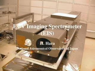
EUV Imaging Spectrometer(EIS) H. Hara National Astronomical Observatory of Japan
Yohkoh, SOHO, and TRACE: reveal dynamic solar corona (flare, plasmoid, jet, coronal expansion …) → Necessity of higher-cadence coronal velocity-field measurements EIS Science Coronal heating Observation with EUV imaging spectrometer (EIS) in emission-line spectroscopy and high-cadence imaging with XRT Energy injection to corona Energy dissipation in corona Photosphere-corona connections Observation with SOT Photospheric motions Flare/CME physics Reconnection physics, Site of large non-thermal line broadening, …
International Collaboration EIS Development team UK Norway MSSL BU RAL Univ. Oslo Japan US NAOJ NASA GSFC JAXA NRL The development started in 1999. The EIS was delivered to JAXA in summer 2003.
Primary Mirror Entrance Filter CCD Camera Front Baffle Grating EIS Optical Layout Primary mirror (offset parabola) S L 1939 mm Slit exchanger Shutter Entrance filter CCD Filter L S 1440mm 1000mm Concave grating
Performance short- band long- band • Large Effective Area in EUV band:170-210 A & 250-290 A Mo/Si multi-layer coated Mirror and Grating High QE CCD: Two 2048×1024 back illuminated CCD • Spatial resolution: 2 arcsec resolution over raster-scan area (1 arcsec pixel sampling) • Line spectroscopy of 20-30 km/s pixel sampling • Instrumental width in emission lines for 1 arcsec slit observation: short- band: 47 mA, long- band: 58 mA • Raster-scan area (EW×NS): 590×512 arcsec2 max. FOV center can move in East-West direction by 890 arcsec. • Wide temperature coverage: log T = 4.7, 5.4, 6.0-7.3 • Simultaneous observation of multiple lines up to 25
EIS Sensitivity Detected photons per 11 area of the sun per 1 sec exposure. AR: active region
w Observables Information from a single emission line • Line intensity • Line shift by Doppler motion • Line width: temperature, non-thermal motion Information from selected two line ratio • Temperature • Density
EIS Slit/Slot • Four slit selections available • Direction of slit length: north-south direction • EUV line spectroscopy - 1 arcsec L arcsec slit for the best quality of image/spectrum quality - 2 arcsec L arcsec slit for a higher throughput • EUV Imaging (Velocity information is convolved.) - 40 arcsec L arcsec slot for imaging with little overlap -266 arcsec L arcsec slot for hunting transient events L > 1024 arcsec (=CCD height)
EIS Field-of-View (FOV) N E W S
EIS Science Targets Bright Point Limb/beyond the limb Active regions/Flares Quiet Sun/ Network brightening Coronal Hole Coronal Hole Boundary Polar Plume S/C re-pointing required
EIS Observations Examples of 240" 240" Raster Scan Discontinuous raster 240 " 240 " 1" slit raster 2" slit raster Wider instrumental width EUV imaging of less contamination by other lines 40" slit raster 266" slit raster (no mirror motion) Contribution of other emission lines
Expected Accuracy of Velocity FL-line (GOES-M2) AR-line AR-line Doppler Velocity Fe XXIV 255 Fe XV 284 Fe XII 195 Line Width Fe XXIV 255 Fe XII 195 Fe XV 284 Number of detected photons (1"1" area)-1
EIS Image Data CCD1 CCD0 height CCD readout height Software window (SW) EIS data size to MDP = total sum of software windows = (window width)i * (window height)i Assemble all SWs Raw data Compression MDP DPCM EIS data of CCSDS format JPEG Compression ratio = compressed data size/ input data size to MDP Data rate ~ [EIS data size to MDP] * [Compression Ratio] / Cadence
EIS Data Flow Data compression DPCM(loss less) or 12bit-JPEG Small spectral window (25 max) CCD Readout Electronics 2Mbps max 1.3 Mbps EIS ICU S/C MDP control 260 kbps max for short duration, 45 kbps average Large hardware CCD window Observation table 1 slit obs. 40 slot obs. 250 slot obs. Spec.width 16 40 250 Spatial width 256 512 256 No. of lines 8 4 4 Compression* 25% 20 % 20% Cadence 3 sec 6 sec 20 sec Rate 42.7 kbps 42.7 kbps 40 kbps Average rate depends on number of downlink stations. Telemetry data format *for 16 bit/pixel data 13 min cadence for 44 rastering
EIS Science Operation • Team core science • Initial science targets • Proposal from users Preparation for EIS SO Merging EIS SO in S/C operation - Obs. table - S/C CMDs EIS Planning EGSE Observation Planning Science ISACS-PLN Feedback Plan approved for EIS operation Feedback Final S/C plan Line selection Exp. duration Compression FOV size etc. Data rate Compression Instrument CAL Check of Obs. Table using PM Outcome Uplink station Analysis Data check Data for analysis Level0 data Level1 data Level2 data Spacecraft Data Reformat EGSE Users Observation in orbit Telemetry Downlink stations JAXA data storage Data centers
Summary • EIS is an excellent instrument to investigate the dynamical solar upper atmospheres. • Scientific output will strongly depend on the EIS observation planning in which ideas of scientists are deeply contained.