Assessing Hydrological Model Performance Using Stochastic Simulation
Assessing Hydrological Model Performance Using Stochastic Simulation. Ke-Sheng Cheng Department of Bioenvironmental Systems Engineering National Taiwan University. INTRODUCTION.


Assessing Hydrological Model Performance Using Stochastic Simulation
E N D
Presentation Transcript
Assessing Hydrological Model Performance Using Stochastic Simulation Ke-Sheng Cheng Department of Bioenvironmental Systems Engineering National Taiwan University
INTRODUCTION • Very often, in hydrology, the problems are not clearly understood for a meaningful analysis using physically-based methods. • Rainfall-runoff modeling • Empirical models – regression, ANN • Conceptual models – Nash LR • Physical models – kinematic wave
Regardless of which types of models are used, almost all models need to be calibrated using historical data. • Model calibration encounters a range of uncertainties which stem from different sources including • data uncertainty, • parameter uncertainty, and • model structure uncertainty.
The uncertainties involved in model calibration inevitably propagate to the model outputs. • Performance of a hydrological model must be evaluated concerning the uncertainties in the model outputs. Uncertainties in model performance evaluation.
ASCE Task Committee, 1993 • “Although there have been a multitude of watershed and hydrologic models developed in the past several decades, there do not appear to be commonly accepted standards for evaluating the reliability of these models. There is a great need to define the criteria for evaluation of watershed models clearly so that potential users have a basis with which they can select the model best suited to their needs”. • Unfortunately, almost two decades have passed and the above scientific quest remains valid.
SOME NATURES OF FLOOD FLOW FORECASTING • Incomplete knowledge of the hydrological process under investigation. • Uncertainties in model parameters and model structure when historical data are used for model calibration. • It is often impossible to observe the process with adequate density and spatial resolution. • Due to our inability to observe and model the spatiotemporal variations of hydrological variables, stochastic models are sought after for flow forecasting.
A unique and important feature of the flow at watershed outlet is its persistence, particularly for the cases of large watersheds. • Even though the model input (rainfall) may exhibit significant spatial and temporal variations, flow at the outlet is generally more persistent in time.
Illustration of persistence in flood flow series A measure of persistence is defined as the cumulative impulse response (CIR).
The flow series have significantly higher persistence than the rainfall series. • We have analyzed flow data at other locations including Hamburg, Iowa of the United States, and found similar high persistence in flow data series.
CRITERIA FOR MODEL PERFORMANCE EVALUATION • Relative error (RE) • Mean absolute error (MAE) • Correlation coefficient (r) • Root-mean-squared error (RMSE) • Normalized Root-mean-squared error (NRMSE)
Coefficient of efficiency (CE) (Nash and Sutcliffe, 1970) • Coefficient of persistence (CP) (Kitanidis and Bras, 1980) • Error in peak flow (or stage) in percentages or absolute value (Ep)
Coefficient of Efficiency (CE) • The coefficient of efficiency evaluates the model performance with reference to the mean of the observed data. • Its value can vary from 1, when there is a perfect fit, to . A negative CE value indicates that the model predictions are worse than predictions using a constant equal to the average of the observed data.
Model performance rating using CE (Moriasi et al., 2007) • Moriasi et al. (2007) emphasized that the above performance rating are for a monthly time step. If the evaluation time step decreases (for example, daily or hourly time step), a less strict performance rating should be adopted.
Coefficient of Persistency (CP) • It focuses on the relationship of the performance of the model under consideration and the performance of the naïve (or persistent) model which assumes a steady state over the forecast lead time. • A small positive value of CP may imply occurrence of lagged prediction, whereas a negative CP value indicates that performance of the considered model is inferior to the naïve model.
ANN model observation An example of river stage forcating Model forecasting CE=0.68466
ANN model observation Naïve model Model forecasting CE=0.68466 CP= -0.3314 Naive forecasting CE=0.76315
Bench Coefficient • Seibert (2001) addressed the importance of choosing an appropriate benchmark series with which the predicted series of the considered model is compared.
The bench coefficient provides a general form for measures of goodness-of-fit based on benchmark comparisons. • CE and CP are bench coefficients with respect to benchmark series of the constant mean series and the naïve-forecast series, respectively.
The bottom line, however, is what should the appropriate benchmark series be for the kind of application (flood forecasting) under consideration. • We propose to use the AR(1) or AR(2) model as the benchmark for flood forecasting model performance evaluation. A CE-CP coupled MPE criterion.
It appears that the model specification error does not affect the parameter uncertainties. However, the bias in parameter estimation of AR(1) modeling will result in a poorer forecasting performance and higher uncertainties in MPE criteria.
ASYMPTOTIC RELATIONSHIP BETWEEN CE AND CP • Given a sample series { }, CE and CP respectively represent measures of model performance by choosing the constant mean series and the naïve forecast series as benchmark series. • The sample series is associated with a lag-1 autocorrelation coefficient .
Given a data series with a specific lag-1 autocorrelation coefficient, we can choose various models for one-step lead time forecasting of the given data series. • Equation [A] indicates that, although the forecasting performance of these models may differ significantly, their corresponding (CE, CP) pairs will all fall on a specific line determined by .
Asymptotic relationship between CE and CP for data series of various lag-1 autocorrelation coefficients.
The asymptotic CE-CP relationship can be used to determine whether a specific CE value, for example CE=0.55, can be considered as having acceptable accuracy. • The CE-based model performance rating recommended by Moriasi et al. (2007) does not take into account the autocorrelation structure of the data series under investigation, and thus may result in misleading recommendations.
Consider a data series with significant persistence or high lag-1 autocorrelation coefficient, say 0.8. Suppose that a forecasting model yields a CE value of 0.55 (see point C). With this CE value, performance of the model is considered satisfactory according to the performance rating recommended by Moriasi et al. (2007). • However, it corresponds to a negative value of CP (-0.125), indicating that the model performs even poorer than the naïve forecasting, and thus should not be recommended.
Asymptotic relationship between CE and CP for data series of various lag-1 autocorrelation coefficients.
1= 0.843 CE=0.686 at CP=0 1= 0.822 CE=0.644 at CP=0 1= 0.908 CE=0.816 at CP=0
For these three events, the very simple naïve forecasting yields CE values of 0.686, 0.644, and 0.816 respectively, which are nearly in the range of good to vary good according to the rating of Moriasi et al. (2007).
In the literature we have found that many flow forecasting applications resulted in CE values varying between 0.65 and 0.85. With presence of high persistence in flow data series, it is likely that not all these models performed better than naïve forecasting.
Another point that worth cautioning in using CE for model performance evaluation is whether it should be applied to individual events or a constructed continuous series of several events. • Variation of CE values of individual events enables us to assess the uncertainties in model performance. Whereas some studies constructed an artifact of continuous series of several events, and a single CE value was calculated from the multiple-event continuous series.
CE value based on such an artifactual series cannot be considered as a measure of overall model performance with respect to all events. • This is due to that fact that the denominator in CE calculation is significant larger for the artifactual series than that of any individual event series, and thus the CE value of the artifactual series will be higher than the CE value of any individual event.
For example, the CE value by naïve forecasting for an artifactual flow series of the three events in Figure 1 is 0.8784 which is significant higher than the naïve-forecasting CE value of any individual event.
1= 0.843 CE=0.686 at CP=0 1= 0.822 CE=0.644 at CP=0 1= 0.908 CE=0.816 at CP=0
A nearly perfect forecasting model CE=0.79021 CE=0.66646 CE=0.79109 CE=0.80027 CE=0.62629 CE=0.77926 CE=0.76404 CE=0.84652 CE=0.85599
A CE-CP COUPLED MPE CRITERION • Are we satisfied with using the constant mean series or naïve forecasting as benchmark? • Considering the high persistence nature in flow data series, we argue that performance of the autoregressive model AR(p) should be considered as a benchmark comparison for performance of other flow forecasting models.