Download
1 / 18
180 likes | 343 Views
A Primer on Atomic Theory Calculations (for X-ray Astrophysicists). F. Robicheaux Auburn University Mitch Pindzola and Stuart Loch. Physical Effects Atomic Structure (wavelength, decay rate, …) Electron Scattering (excitation, ionization, …). Physical Effects: mean field.

E N D
A Primer on Atomic Theory Calculations (for X-ray Astrophysicists) F. Robicheaux Auburn University Mitch Pindzola and Stuart Loch • Physical Effects • Atomic Structure (wavelength, decay rate, …) • Electron Scattering (excitation, ionization, …)
Physical Effects: mean field Electrons screen the charge of nucleus. Near nucleus V decreases faster than -kZe2/r Low l see deeper potential and are more deeply bound actual 3s is more strongly bound than 3p which is more strongly bound than 3d
Physical Effects: correlation The main interaction between two electrons is through V(r1,r2) = k e2/|r1 – r2| 2 electrons can exchange energy & angular momentum 2p61S mixes “strongly” with 2p43d21S but “weakly” with 2p23d41S 2s2p62S can decay into 2s22p4Ed 2S (auto-ionization)
Physical Effects: Relativity Spin-orbit interaction Mass-velocityKE = p2/2m – p4/8m3c2 + … Darwin termDirac equation ~ spread electron over distance ~h/mc Quantum Electro-Dynamics effectsSelf energy, vacuum polarization, Breit interaction
Structure: Hartree/Dirac-Fock Approximate the wave function by single antisymmetrized wave function. Example: 1s21S Y(1,2)=R10(r1)Y00(W1) R10(r2)Y00(W2) (h1i2 – i1h2)/21/2 Equation for unknown function determined by variational principle. No correlation! Difficulties Equations are nonlinearOnly E variational Advantages Well developed programsFastFix by better calcs
Structure: Perturbation Theory Corrections to wave function can be small. Example: 1s21S + 2s21S + 3s21S + … Ea = <a|H|a> + Sb |<a|DH|b>|2/(Ea,0 – Eb,0) + … 0th order states determined by “simple” H.Numerical calculation of matrix elements Difficulties Not available for most statesStrong effects Advantages Well developed programsCan be very, very accurateHigher order correlations
Structure: MCHF/MCDF Approximate the wave function by superposition of antisymmetrized wave functions. Example: 1s21S + 2s21S Y(1,2)=[C1R10(r1)R10(r2) + C2R20(r1)R20(r2)] (L=0,S=0) Equation for unknown functions and coefficients determined by variational principle. Difficulties Equations are nonlinearSolve 1 state at a timeMainly for deep states Advantages Well developed programsCan be very accurateFewest terms in sum
Structure: R-matrix Approximate the wave function by superposition of antisymmetrized wave functions. Example: 1s21S + 2s21S Y(1,2)=[C1R10(r1)R10(r2) + C2R20(r1)R20(r2)] (L=0,S=0) Functions found outside but coefficients determined by variational principle. Difficulties Many basis functionsSmall/large corrections treated same Advantages Well developed programsCan be very accurateEquations are linear
Structure: Mixed CI & perturbative Use configuration interaction method to include some effects. Use perturbation theory to include other effects. Examples: Non-relativistic CI – mass-velocity, S.O., Darwin Relativistic CI – Q.E.D. Difficulties May not be accurate enoughNot full pert. potential Advantages Complicated interaction included
Structure: Transitions Radiative decay computed using transition matrix elements. Transition matrix elements are not variational.Electric dipole allowed transitions are typically strongest. Beware Spin changing transitions (2s2p 3P1g 2s21S0)Dipole forbidden transitions (3d g 2s)Two electron transitions (2p3d 1P g 2s21S)Nearly degenerate states !!!!! 0 !!!!!
e- Scattering: Non-resonant Pert. Th. Direct transition of target from initial to final state Example: (1s21S) Ep 2P g (1s2p 3P) Es 2P Transition amplitude approximated Tf f i = <yf(0)|V|yi(0)> Plane wave Born No potential for continuumDistorted wave Born Avg potential for continuum Difficulties No resonancesStrong couplingWhich average potential? Advantages FastAccurate for ionsMore accurate target states
e- Scattering: Resonant Pert. Th. Direct & indirect transitions of target Example:(1s21S) Ep 2P n 1s3s3p 2P n (1s2p 3P) Es 2P Transition amplitude approximatedTf f i = <yi(0)|V|yf(0)> + Sn V(0)fn [E – En + i Gn/2]-1 V(0)ni What potential to use for bound and continuum states?Interference and interaction through continuum? Difficulties Strong couplingWhich average potential?Inaccurate bound states Advantages FastFix by better calcsEasy averaging
e- Scattering: R-matrix Variational calculation for log-derivative at boundary Basis set expansion of Hamiltonian in small region Rij = ½ Sn yin yjn /(E – En) Analytic or numerical function take RgT Long range interaction through integration/perturbationDiagonalize matrix once for each LSJp Difficulties Less accurate targetPseudo-resonancesFine energy mesh Advantages Accurate channel couplingRadiation damp. & relativityPseudo-states for ionization
e- Scattering: Other close-coupling Special purpose close coupling methods can be very accurate for specific problems. Important for testing more heavily used methods & experiment. Convergent close coupling (CCC)-solve Lippman-Schwinger equation using basis set technique Time dependent close coupling (TDCC)-solve the time dependent Schrodinger equation (usually grid of points) Hyperspherical close coupling (HSCC)-solve for the time independent wave function using hyperspherical coords
e- Scattering Example: Excitation Excitation cross section directly used in computing the radiated power. Li in electron plasma ne = 1010 cm-3 dotted—PWB dashed—DWB solid—RMPS Li Li2+ Li+ Perturbation theory worse for neutral. DWB not that bad. Thermodynamics can help less accurate calcs.
e- Scattering Example: Ionization Average over l blue dashed—DWB green dot-dashed—CTMC red solid—RMPS Perturbation theory worse for higher n-states. CTMC does not quickly improve with n DWB does better for ionization of Li2+
e- Scattering Example: DR of N4+ Glans et al, PRA 64,043609 (2001). Details of 1s22p5l Upper 4 calcs use exptl 2s-2pj splittings Bottom graph: diagonalization+pert Low T might have problems Hard work for 2 active electrons all orders pert theor
Concluding Remarks “Must” use CI/CC or mixed methods (CI+pert) for neutrals and near neutrals. Scattering from “highly” excited atoms very difficult but errors may not be important. Typical weak transitions are less accurate than typical strong transitions. Photo-recombination can be abnormally sensitive at low temperatures if low lying resonances are present. Ionization in neutrals and near neutrals is difficult. AMO + plasma modeling needed for practical error est.