Download
1 / 49
550 likes | 835 Views
Understand advanced econometric models including VAR models, cointegration, and VEC models. Learn about the dynamic nature of economic processes and lag structures in models. Explore the Lüdeke consumption and investment functions for Germany. Gain insights into multiplicators and ADL models in econometrics.

E N D
Advanced Econometrics - Lecture 6Multivariate Time Series Models
Advanced Econometrics - Lecture 6 • Econometric Models • Multiplicators and ADL Models • Cointegration • VAR Models • Cointegration and VAR Models • Vector Error-Correction Model • Estimation of VEC Models Hackl, Advanced Econometrics, Lecture 6
The Lüdeke Model for Germany Consumption function Ct = α1 + α2Yt + α3Ct-1 + ε1t Investment function It = β1 + β2Yt + β3Pt-1 + ε2t Import function Mt = γ1 + γ2Yt + γ3Mt-1 + ε3t Identity relation Yt = Ct + It - Mt-1 + Gt with C: private consumption, Y: GDP, I: investments, P: profits, M: imports, G: governmental spendings endogenous: C, Y, I, M exogenous: G, P-1 Hackl, Advanced Econometrics, Lecture 6
Econometric Models • Basis is the multiple linear regression model • Model extensions • Dynamic models • Systems of regression relations Hackl, Advanced Econometrics, Lecture 6
Dynamic Models: Examples • Demand model: describes the quantity Q demanded of a product as a function of its price P and the income Y of households • Demand is determined by • Current price and current income (static model): • Qt = β1 + β2Pt + β3Yt + εt • Current price and income of the previous period (dynamic model): • Qt = β1 + β2Pt + β3Yt-1 + εt • Current price and demand of the previous period (dynamic autoregressive model): • Qt = β1 + β2Pt + β3Qt-1 + εt Hackl, Advanced Econometrics, Lecture 6
The Dynamic of Processes • Static processes: immediate reaction to changes in regressors, the adjustment of the dependent variables to the realizations of the independent variables will be completed within the current period, the process seems to be always in equilibrium • Static models are inappropriate • Some processes are determined by the past, e.g., energy consumption depends on past investments into energy-consuming systems and equipment • Actors in economic processes may respond delayed, e.g., time for decision-making and procurement processes exceeds the observation period • Expectations: e.g., consumption depends not only on current income but also on the income expectations; modeling the expectation may be based on past development Hackl, Advanced Econometrics, Lecture 6
Elements of Dynamic Models • Lag structures, distributed lags: they describe the delayed effect of one or more regressors on the dependent variable; e.g., the distributed lag of order s, the DL(s) model, is • Yt = δ + Σsi=0φiXt-i + εt • Geometric or Koyck lag structure: infinite lag structure with • φi = λ0λi • ADL models: autoregressive model with lag structure, e.g., the ADL(1,1) model • Yt = δ + θYt-1 + φ0Xt + φ1Xt-1 + εt • Error correction model: • ΔYt = - (1-θ)(Yt-1 - α - βXt-1)+ φ0ΔXt + εt • which is obtained from the ADL(1,1) model with α = δ/(1-θ) and β = (φ0+φ1)/(1- θ) Hackl, Advanced Econometrics, Lecture 6
Advanced Econometrics - Lecture 6 • Econometric Models • Multiplicators and ADL Models • Cointegration • VAR Models • Cointegration and VAR Models • Vector Error-Correction Model • Estimation of VEC Models Hackl, Advanced Econometrics, Lecture 6
Example: Consumption Function Data for Austria (1976:1 – 1995:2), logarithmic differences: Ĉ = 0.009 + 0.621Y with t(Y) = 2.288, R2 = 0.335 DL(2) model, same data: Ĉ = 0.006 + 0.504Y – 0.026Y-1+ 0.274Y-2 with t(Y) = 3.79, t(Y-1) = – 0.18, t(Y-2) = 2.11, R2 = 0.370 Effect of income on consumption: • Short term effect, i.e. effect in the current period: ΔC = 0.504, given a change in income ΔY = 1 • Overall effect, i.e., cumulative current and future effects ΔC = 0.504 – 0.026 + 0.274 = 0.752, given a change in income ΔY = 1 Hackl, Advanced Econometrics, Lecture 6
Multiplicators Describe the effect of a change in explanatory variable X by ΔX = 1 on current and future values of the dependent variable Y • DL(s) model: Yt = δ + φ0Xt + φ1Xt-1 + … + φsXt-s + εt • short run or impact multiplier: effect of the change in the same period (ΔY = φ0) • long run or equilibrium multiplier: the effect of ΔX = 1, cumulated over all future (ΔY = φ0 + … + φs) • ADL(1,1) model: Yt = δ + θYt-1 + φ0Xt + φ1Xt-1 + εt • impact multiplier: ΔY = φ0; after one period: ΔY = θφ0 + φ1; after two periods: ΔY = θ(θφ0 + φ1); etc. • equilibrium multiplier: φ0 + (θφ0 + φ1) + θ(θφ0 + φ1) + … = (φ0 + φ1)/(1 – θ) Hackl, Advanced Econometrics, Lecture 6
Multiplicators, cont’d Describe the effect of a change in explanatory variable X on current and future values of Y • ADL(1,1) model written as error correction model ΔYt = -(1-θ)(Yt-1 - α - βXt-1)+ φ0 ΔXt + εt effects on ΔY • due to changes ΔX • due to equilibrium error, i.e., Yt-1 - α - βXt-1, a negative adjustment -(1-θ)(Yt-1 - α - βXt-1) Hackl, Advanced Econometrics, Lecture 6
The ADL(p,q) Model ADL(p,q): generalizes the ADL(1,1) model: θ(L)Yt = δ + Φ(L)Xt + εt with lag polynomials θ(L) = 1 - θ1L - … - θpLp , Φ(L) = φ0 + φ1L + … + φqLq Given invertibility of θ(L), i.e., θ1 + … + θp < 1, Yt = θ(1)-1δ + θ(L)-1Φ(L)Xt + θ(L)-1εt The coefficients of θ(L)-1Φ(L) describe the dynamic effects of X on current and future values of Y • equilibrium multiplier ADL(0,q): coincides with the DL(q) model; θ(L) = 1 Hackl, Advanced Econometrics, Lecture 6
Partial Adjustment Model Describes the process of adapting to a desired or planned value Example: Stock level K and revenues S • The desired (optimal) stock level K* depends of the revenues S K*t = α+ βSt + ηt • Actual stock level Kt deviates from K*t • (Partial) adjustment according to Kt – Kt-1 = (1 - θ)(K*t – Kt-1) with 0 < θ < 1 • Substitution for K*t gives the AR form of the model Kt = Kt-1 + (1 - θ)α + (1 - θ)βSt - (1 - θ)Kt-1+ (1 – θ)ηt = δ + θKt-1 + φ0St + εt which is a ADL(1,0) model Hackl, Advanced Econometrics, Lecture 6
Advanced Econometrics - Lecture 6 • Econometric Models • Multiplicators and ADL Models • Cointegration • VAR Models • Cointegration and VAR Models • Vector Error-Correction Model • Estimation of VEC Models Hackl, Advanced Econometrics, Lecture 6
The Drunk and her Dog M. P. Murray, A drunk and her dog: An illustration of cointegration and error correction. The American Statistician,48 (1997), 37-39 drunk: xt – xt-1 = ut dog: yt – yt-1 = wt Cointegration: xt–xt-1 = ut+c(yt-1–xt-1) yt–yt-1 = wt+d(xt-1–yt-1) Hackl, Advanced Econometrics, Lecture 6
A Macro-Economic Example I(1) variables • M: money stock • P: price level • Y: output • R: nominal interest rate Equilibrium relation (in logarithms) m - p = γ0 +γ1y + γ2r, γ1> 0; γ2 < 0 Theory implies that x’β = (m, p, y, r) (1, -1, - γ1, - γ2)’ = m - p -γ1y - γ2r ~ I(0) Deviations from the equilibrium are corrected Hackl, Advanced Econometrics, Lecture 6
Notation Non-stationary variables X, Y: Xt~ I(1), Yt~ I(1) exists β such that Zt = Yt - βXt ~ I(0) • Xt and Yt are cointegrated, have a common trend • β is the cointegration parameter • (1, - β)’ is the cointegration vector Cointegration implies a long-run equilibrium Hackl, Advanced Econometrics, Lecture 6
Long-run Equilibrium Equilibrium defined by Yt = α + βXt Equilibrium error: zt = Yt - βXt - α = Zt - α • zt~ I(0): equilibrium error stationary, fluctuating around zero • Yt, βXt not integrated: • zt~ I(1), non-stationary process • Yt = α + βXt does not describe an equilibrium Cointegration vector implies a long-run equilibrium relation Hackl, Advanced Econometrics, Lecture 6
Identification of Cointegration Information about cointegration: • Economic theory • Visual inspection of data • Statistical test Hackl, Advanced Econometrics, Lecture 6
Testing for Cointegration Non-stationary variables Xt~ I(1), Yt~ I(1) Yt = α + βXt + εt • Xt and Yt are cointegrated: εt~ I(0) • Xt and Yt are not cointegrated: εt~ I(1) Tests for cointegration: • If β is known, unit root test based on differences Yt - βXt • Unit root test based on residuals et Δet = γ0 + γ0et-1 + ut Critical values, Verbeek, Tab. 9.2 • Cointegrating regression Durbin-Watson (CRDW) test: DW statistic from OLS-fitting Yt = α + βXt + εt Critical values, Verbeek, Tab. 9.3 Hackl, Advanced Econometrics, Lecture 6
OLS Estimation To be estimated: Yt = α + βXt + εt cointegrated non-stationary processes Yt~ I(1), Xt~ I(1) εt~ I(0) OLS estimator b for β • Non-standard distribution • Super consistent: • T(b – β) converges to zero • In case of consistency: √T(b – β) converges to zero • Robust • Non-normal; e.g., t-test misleading • Small samples: bias Hackl, Advanced Econometrics, Lecture 6
OLS Estimation, cont’d To be estimated: Yt = α + βXt + εt non-stationary processes Yt~ I(1), Xt~ I(1) If εt~ I(1), i.e., Yt and Xt not cointegrated: spurious regression OLS estimator b for β • Non-standard distribution • High values of R2, t-statistic • Highly autocorrelated residuals • Low value of DW statistic Hackl, Advanced Econometrics, Lecture 6
Error-correction Model Granger’s Representation Theorem (Engle & Granger, 1987): If a set of variables is cointegrated then an error-correction relation of the variables exists non-stationary processes Yt~ I(1), Xt~ I(1) with cointegrating vector (1, -β)’: error-correction representation θ(L)ΔYt = δ + Φ(L)ΔXt-1 - γ(Yt-1– βXt-1) + α(L)εt with lag polynomials θ(L) – with θ0=1 –, Φ(L), and α(L) E.g., ΔYt = δ + φ1ΔXt-1 - γ(Yt-1– βXt-1) + εt Error-correction model: describes • the short-run behavior • consistent with the long-run equilibrium Converse statement: if Yt~ I(1), Xt~ I(1) have an error-correction representation, they are cointegrated Hackl, Advanced Econometrics, Lecture 6
Advanced Econometrics - Lecture 6 • Econometric Models • Multiplicators and ADL Models • Cointegration • VAR Models • Cointegration and VAR Models • Vector Error-Correction Model • Estimation of VEC Models Hackl, Advanced Econometrics, Lecture 6
The VAR(p) Model VAR(p) model: generalization of the AR(p) model for k-vectors Yt Yt = δ + Θ1Yt-1 + … + ΘpYt-p + εt with k-vectors Yt, δ, and εt and kxk-matrices Θ1, …, Θp Shorter: Θ(L)Yt = δ + εt with Θ(L) = I – Θ1L - … - ΘpLp Error terms εt have covariance matrix Σ; allows for contemporary correlation In deviations yt = Yt – μ, with μ= E{Yt} = (I – Θ1 - … - Θp)-1δ = Θ(1)-1δ Θ(L)yt = εt MA representation: Yt = μ + Θ(1)-1εt = μ + εt + A1εt-1 + A2εt-2 + … Hackl, Advanced Econometrics, Lecture 6
Example: Income and Consumption Model: Yt = δ1 + θ11Yt-1 + θ12Ct-1 + ε1t Ct = δ2 + θ21Ct-1 + θ22Yt-1 + ε2t With Z = (Y, C)‘, 2-vectors δ and ε, and (2x2)-matrix Θ, the VAR(1) model is Zt = δ + ΘZt-1 + εt Represents each component of Z as a linear combination of lagged variables Hackl, Advanced Econometrics, Lecture 6
Income and Consumption, cont’d AWM data base, 1970:1-2003:4: PCR (real private consumption), PYR (real disposable income of households); respective annual growth rates: C, Y Fitting Zt = δ + ΘZt-1 + εtwith Z = (Y, C)‘ gives with AIC = -14.45; VAR(2) model: AIC = -14.43 Compare: consumption function Ĉ = 0.011 + 0.718Y with t(Y) = 15.55, adj.R2 = 0.65, and AIC = -6.61 Hackl, Advanced Econometrics, Lecture 6
VAR Models: Advantages Besides the generality of the specification: • Meets assumptions of OLS estimation • Requires no distinction between endogenous and exogenous variables (which is always arbitrary) • Allows for non-stationarity and cointegration The number of parameters to be estimated grows rapidly with p and k Number of components of Θ for some values of p and k Hackl, Advanced Econometrics, Lecture 6
Advanced Econometrics - Lecture 6 • Econometric Models • Multiplicators and ADL Models • Cointegration • VAR Models • Cointegration and VAR Models • Vector Error-Correction Model • Estimation of VEC Models Hackl, Advanced Econometrics, Lecture 6
VAR(p) Model, Stationarity and Cointegration VAR(p) process • is stationary, if all roots zi of the characteristic polynomial Θ(L), det Θ(z) = 0, fulfill |zi| > 1; det Θ: determinant of Θ(.) For kxk-matrices Θ1,…, Θp: kp roots • is non-stationary, if zi = 1 is a (multiple) root of the characteristic polynomial Θ(L) For non-stationary variables with the same order of integration, cointegrating relationships may exist Hackl, Advanced Econometrics, Lecture 6
VAR(1) Model and k=2 VAR(1) model for 2-vector yt: characteristic polynomial Θ(L) for Θ(z) = I – Θz has 2 roots; three cases • If both roots of det Θ(z) = 0 have value one, then both variables in y integrated, no cointegrating relationship between them • If exactly one of the two roots has value one, then the variables cointegrated • If none of the roots has value one, both variables are stationary, no cointegrating relationship Hackl, Advanced Econometrics, Lecture 6
Example Model for Y and Y: Xt + αYt = u1t, u1t = ρ1u1,t-1 + ε1t (A) Xt + βYt = u2t, u2t = ρ2u2,t-1 + ε2t (B) with α≠b, independent IID(0,si2)-processes εi, i = 1,2 Reduced forms for Y and Y: linear combinations of the ui VAR(1) model Xt = (ρ1 – αδ)Xt-1 – αβδYt-1 + v1t Yt = δXt-1 + (ρ1 + βδ)Yt-1 + v2t with δ = (ρ1 – ρ2)/(α – β) and linear combinations vi of the εi Characteristic polynomial det Θ(z) = 1 – z(ρ1 – ρ2) + z2ρ1ρ2 = 0 has characteristic roots z1 = 1/ρ1 and z2 = 1/ρ2 Hackl, Advanced Econometrics, Lecture 6
Example, cont’d • Let ρ1 = 1, |ρ2| <1, i.e., u1 ~ I(1), u2 ~ I(0), then z1 = 1, z2 > 1; the reduced forms imply X ~ I(1) and Y ~ I(1), i.e., both are non-stationary, equation (B) indicates cointegration of X and Y; see case b) • |ρ1| <1, |ρ2| <1; i.e., u1 ~ I(0), u2 ~ I(0), also X ~ I(0) and Y ~ I(0); all are stationary; see case c) • Let ρ1 = ρ2 = 1, i.e., u1 ~ I(1), u2 ~ I(1), both are non-stationary, also X and Y are non-stationary, no cointegrating relation between X and Y; see case a) Hackl, Advanced Econometrics, Lecture 6
VAR(p) Model: Cointegration VAR(1) model for k-vector yt: characteristic polynomial Θ(L) for Θ(z) = I – Θz has k roots • if k-r roots of the characteristic polynomial det Θ(z) = 0 have the value one, then r cointegrating relationships exist between the variables of yt Hackl, Advanced Econometrics, Lecture 6
Example, cont’d Case ρ1 = 1, |ρ2| <1: differences ΔXt = – αδXt-1 – αβδYt-1 + v1t ΔYt = δXt-1 + βδYt-1 + v2t In matrix notation with Z = (X,Y)’: going from Zt = ΘZt-1 + δ + εt to differences gives ΔZt = - (I – Θ)Zt-1 + δ + εt = - Θ(1)Zt-1 + δ + εt with Hackl, Advanced Econometrics, Lecture 6
Advanced Econometrics - Lecture 6 • Econometric Models • Multiplicators and ADL Models • Cointegration • VAR Models • Cointegration and VAR Models • Vector Error-Correction Model • Estimation of VEC Models Hackl, Advanced Econometrics, Lecture 6
Granger‘s Representation Theorem VAR(1) model: yt = Θ1yt-1 + δ + εt, in differences with Θ(L) = I - Θ1L Δyt = - Θ(1)yt-1 + δ + εt r{Θ(1)}: rank of Θ(1), cointegrating rank • If r{Θ(1)} = 0, then Δyt = δ + εt, i.e., y is a k-dimensional random walk, each component is I(1), no cointegrating relationship • If r{Θ(1)} = r < k, there is a (k - r)-fold unit root, (kxr)-matrices γ and β can be found, both of rank r, with Θ(1) = γβ'the r columns of β are the cointegrating vectors of r cointegrating relations (β in standardized form, i.e., the main diagonal elements of β are ones) • If r{Θ(1)} = k, VAR(1) process is stationary, all components of y are I(0) Hackl, Advanced Econometrics, Lecture 6
Vector Error-Correction Model VAR(1) model Δyt = - Θ(1)yt-1 + δ + εt Θ(1) = γβ'with r{Θ(1)} = r < k • Δyt is stationary • β'yt is stationary, each of the r columns of β defines a cointegrating relation yt consists of k-r independent deterministic and r independent stochastic trends Vector error-correction model, VEC model (VECM) Δyt = - γβ'yt-1 + δ + εt • Cointegrating rank r • γ: Adaptation parameters Hackl, Advanced Econometrics, Lecture 6
Example, cont’d Case ρ1 = 1, |ρ2| <1: Standardized form: π = (1, β)’ Cointegrating relation: π’yt-1 = Xt-1 + βYt-1 Hackl, Advanced Econometrics, Lecture 6
The VEC(1) Model VAR(1) model yt = Θ1yt-1 + δ + εt in form of the VEC model Δyt = - γβ'yt-1 + δ + εt with cointegrating rank r describes changes Δyt as function of • the intercept vector δ • of r equilibrium relations Deviations from equilibrium in period t -1 are partly corrected in period t by - γβ'yt-1 adaptation parameters (elements of matrix γ) indicate the proportion of the correction, are a measure of the correction speed Hackl, Advanced Econometrics, Lecture 6
The VEC(p) Model Extension of the VAR(1) process for the k-vector yt to Θ(L) yt = δ + εt with Θ(L) = I – Θ1L - … - ΘpLp For r{Θ(1)} = r < k Θ(L) = – Θ(1) L + (1 – L)Γ(L) with Θ(1) = γβ' the VAR(p) model can be written as Δyt = - Γ1Δyt-1 - … - ΓpΔyt-p - γβ'yt-1 + δ + εt Columns of β are cointegrating vectors, define r cointegrating relations Example: VAR(2) process yt = Θ1yt-1 +Θ2yt-2 +δ + εt results in Δyt = Γ1Δyt-1 + Πyt-1 + δ + εt with Γ1 = (-Θ2), Π = - (I - Θ1 - Θ2) = - Θ(1) Hackl, Advanced Econometrics, Lecture 6
Advanced Econometrics - Lecture 6 • Econometric Models • Multiplicators and ADL Models • Cointegration • VAR Models • Cointegration and VAR Models • Vector Error-Correction Model • Estimation of VEC Models Hackl, Advanced Econometrics, Lecture 6
Estimation of VEC Models Assumption: k-vector yt~ I(1) Estimation of the parameters: • Specification of intercepts and deterministic trends • in the components of yt and • in the cointegrating relations • Choice of the cointegrating rank r, R3-method of Johansen • Estimation of the cointegrating relations, standardizing • Estimation of the VEC model Hackl, Advanced Econometrics, Lecture 6
Johansen‘sR3 Methode Reduced rank regression or R3 method, also Johansen's test: an iterative method for specifying the cointegrating rank r The test is based on the k eigenvalues λi (λ1> λ2>…>λk) of Y1‘Y1 – Y1ΔY(ΔY‘ΔY)-1ΔY‘Y1, with ΔY: (Txk) matrix of differences Δyt, Y1: (Txk) matrix of yt-1 • if r{Θ(1)} = r, the k-r smallest eigenvalues obey: log(1- λi) = 0 Iterative test procedures • Trace test • Maximum eigenvalue test or max test Hackl, Advanced Econometrics, Lecture 6
Tests LR tests, based on the assumption of normally distributed errors • Trace test: for r0 = 0, 1, …, test of H0: r ≤ r0 against H1: r > r0 λtrace(r0) = - T Σkj=r0+1log(1-Îj) Îj: estimator of λj Stops when H0 is rejected for the first time Critical values from simulations • Max test: tests for r0 = 0, 1, …: H0: r = r0 against H1: r = r0+1 λmax(r0) = - T log(1 -Îr0+1) Stops when H0 is rejected for the first time Critical values from simulations Hackl, Advanced Econometrics, Lecture 6
Example: Income and Consumption Model: Yt = δ1 + θ11Yt-1 + θ12Ct-1 + ε1t Ct = δ2 + θ21Ct-1 + θ22Yt-1 + ε2t With Z = (Y, C)‘, 2-vectors δ and ε, and (2x2)-matrix Θ, the VAR(1) model is Zt = δ + ΘZt-1 + εt Represents each component of y as a linear combination of lagged variables Hackl, Advanced Econometrics, Lecture 6
Income and Consumption, cont’d AWM data base: PCR (real private consumption), PYR (real disposable income of households); logarithms: C, Y • Check whether C and Y are non-stationary: C ~ I(1), Y ~ I(1) • Johansen test for cointegration: given that C and Y have no trends and the cointegrating relationship has an intercept: r = 1 (p <0.05) the cointegrating relationship is C = 8.55 – 1.61Y with t(Y) = 18.2 Hackl, Advanced Econometrics, Lecture 6
Income and Consumption, cont’d • VEC(1) model (same specification as in 2.) Dyt = - γ(β'yt-1 + δ) + ΓDyt-1 + εt The model explains growth rates of PCR and PYR; AIC = -15.41 is smaller than that of the VAR(1)-Modell (AIC = -14.45) Hackl, Advanced Econometrics, Lecture 6
Exercise Answer questions a. to f. of Exercise 9.3 of Verbeek Hackl, Advanced Econometrics, Lecture 5