Download
1 / 18
190 likes | 255 Views
Explore LTspice, a powerful SPICE simulation program for circuit design. Learn how to create circuits, analyze waveform, and simulate components. Download your free copy today!

E N D
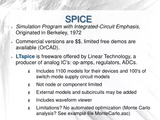
SPICE • Simulation Program with Integrated-Circuit Emphasis, Originated in Berkeley, 1972 • Commercial versions are $$, limited free demos are available (OrCAD). • LTspice is freeware offered by Linear Technology, a producer of analog IC's: op-amps, regulators, ADCs. • Includes 1100 models for their devices and 100's of switch-mode supply circuit models • Not node or component limited • External models and subcircuits may be added • Includes waveform viewer • Limitations? No automated optimization (Monte Carlo analysis? See example file MonteCarlo.asc)
SPICE Demonstration - LTspice • What is LTspice and what can you do with it? • Circuit simulation: extendable parts libraries; built-in diode and transistor behavioral models • Draw a circuit (schematic capture) • Create a BOM • Where to get a free copy of Ltspice? • Go to http://www.linear.com/LTspice • Left click on “Download LTspice IV” • How to learn to use it:LTspice IV Getting Started Guide
SPICE Text Listing SPICE originally required a text based input. Remember punch cards anyone? Now, the graphical capture front end automatically creates the necessary node and command lists. Listing here is from the simple linear supply design. Each circuit node in your design is automatically numbered and can be renamed. Example syntax for transistor: Qxxx Collector Base Emitter [Substrate Node] model * C:\Users\Steve\Desktop\SPICE Demonstration\SimpleSupply.asc Q1 N001 N003 Vout 0 2N3055 R1 N003 N002 {10k-Pres} R4 0 N003 {Pres} R2 N001 N002 820 R3 Vout 0 {Rload} C3 Vout 0 470µF V1 N001 N004 20 D1 0 N002 BZX84C15L I1 Vout 0 PULSE(1mA 50mA 10ms 10ns 10ns 100ms 500ms 1) C2 Vout N001 .02pf V2 N004 0 SINE(0 2 120 0 0 0 20) .model D D .lib C:\PROGRA~2\LTC\LTSPIC~1\lib\cmp\standard.dio .model NPN NPN .model PNP PNP .lib C:\PROGRA~2\LTC\LTSPIC~1\lib\cmp\standard.bjt .PARAM Rload=970 .dc I1 10mA 100mA 2mA ;tran 0 200ms 0 .step param Pres 1k 9k 1k * .step temp -40 80 15 .param Pres=5k .backanno .end
SPICE Prefixes and Suffixes From Ltspice Help
Power Supply Example 20V 2N3055 60Vceo 10A 15V *My assumptions in Blue
Simulation Types • Transient Analysis (.tran) • User sets starting conditions and runs the simulation for a specified time. • Output graphs show voltages/currents as a function of time • DC Analysis (.dc) • Shows the DC operating point while a voltage or current source is stepped through the specified range. • AC Analysis (.ac) • A voltage or current symbol is the source for the circuit exitation specified as a frequency range. • Output graphs are a log scale (dB) voltage or current function of frequency. • There is also “Noise”, “DC Operating Point”, and “DC Transfer Function”
LTspice Simulation Demo capture of the following design: SimpleSupply.asc To simplify, the transformer and rectifier are replaced with a voltage source V1. Represent a potentiometer with two resistors and use of a “parameter”.
What makes a good power supply? • An ideal supply is a voltage source with zero Output Resistance • The output voltage should be stable as Temperature changes • The output voltage should be stable if the Output Current changes suddenly. • The output voltage should be independent of Input Power Fluctuations • Are all supply components operating within their limits for voltage, current, and power dissipation? • This really is true for any design...
Output Resistance? • Use .DC Analysis with a current source to vary the load • Attach 2 cursors to the output voltage trace and measure the change in voltage and current. • Up/Down cursor keys moves between traces. Right click on cursor to display step information. • Rout = deltaV / delta I • Test at multiple output voltage settings (“.step” with parameters) Why is the output resistance worse (higher) in the middle of the pot travel?
Temperature Effect on Output? • Use .temp or “.step temp” with .DC Analysis to see how the output voltage changes with temperature • From -40C to +80C, the output shifts about 0.4V, or about 3.3mV per degree C. • What is causing this? (hint:PN junctions) +80C -40C -4 -40F
Stable with Output Current Changes? • Add a Current Source in “Pulse” mode to vary load current • Use .tran Analysis • Curves show the effect of a short (90ms) spike of 50mA in output current. • Aside from voltage droop due to non-zero output resistance, no sign of ringing or other instability.
Input Source Rejection? 39mVp-p • We know that the AC source (transformer and rectifier) will produce a 120Hz ripple on the input to the series transistor. • Add a second voltage source to simulate 120 Hz ripple, set to 4Vp-p (just a guess). • Use .tran to measure effect on output. (.AC analysis could be used, too). • Worst rejection 40dB (top) high output voltage and large load current (50mA). • Best rejection 65dB (bottom) low output voltage and low load current (1mA). 2.2mVp-p
Waveform Viewer • Click any node to display voltage waveform (cursor is a red voltage probe) • Click and hold any node (red probe appears) then drag to another node and release when black probe appears. Displays voltage difference between the selected nodes. • Hover over any symbol lead until current probe appears and Click. Current waveform is displayed. • Hold Alt key and hover over a component. Click the thermometer symbol for power waveform display. • On Waveform Display • Cursor position appears in bottom frame. • Drag a box and hold – Box limits appear in bottom frame. • Drag a box and click – display zooms. • Left click on node name – select # of cursors • Right click on node name – cursor is attached to waveform and info box appears. Drag cursors as desired. • Hold Ctrl key and right click node name – Average value for displayed range is calculated and appears. • The FFT of any signal can be displayed: under VIEW menu • Many more... The help is actually rather helpful!
Modified Circuit #1 • Reduce resistance “seen” by Q1 Base by adding Q2 emitter follower. • Output resistance now <1.5 ohms (was 37 ohms) • Still stable with output current change. • Input source rejection is much better: now 55dB worst case vs. 40dB, but... • Larger temperature sensitivity: 5.1mV/C vs. 3.3mV/C • Likely worth the trade-off!
What about the Transformer and Rectifier?? • The simulation runs faster as demonstrated with fewer components. • Transformer model parameters would have to be measured for accuracy - not given in datasheets. • Nevertheless, to model a transformer: • draw multiple inductors, set inductance and series resistance. Note: inductance ratio is square of turns ratio. • Link inductors with Mutual Inductance SPICE directive, eg. “K L1 L2 0.98” links L1 and L2 with a 0.98 coupling coefficient. • Note the appearance of phasing dots. • See Model: Transformer and Rectifier.asc
One Last Improved Version • Circuit Source: Bob Pease, Troubleshooting Analog Circuits, 1991 • Output resistance is 72 micro-ohms! • Stable with output current change +50mA. • Input source rejection is better: now 58dB worst case • Temperature sensitivity virtually undetectable: 5mV TOTAL! • R1 sets the output current limit, ~300mA. • Lack of output capacitor protects circuit under test - low discharge energy
.AC Frequency Analysis • To demonstrate .AC analysis, the following model shows 2 independent filters • Source: Hayward et al. Experimental Methods in RF DESIGN, 2009 pg 8.14
Last Word • LTspice is a very useful tool. • See “LTC/LTspiceIV/examples/Educational” folder for useful examples • Most Linear Technology components provide “test fixtures”, ready to run macromodels. • Like any tool, results are only as good as the inputs (models). • In SPICE, wires have zero resistance, capacitors, inductors, and resistors are ideal. • Real components (even passives) have stray capacitance and inductance, as well as non-linear behavior. • Any circuit design must be built and tested on the bench to verify function.