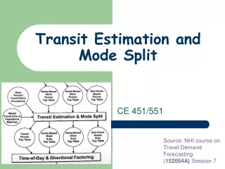
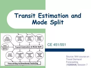
Transit Estimation and Mode Split
Transit Estimation and Mode Split. CE 451/551. Source: NHI course on Travel Demand Forecasting ( 152054A) Session 7. Terminology. HOV Light Rail Portland ; Florence Heavy rail Commuter rail Local bus service Express bus service Paratransit service Busways Headways/frequency

Transit Estimation and Mode Split
E N D
Presentation Transcript
Transit Estimation and Mode Split CE 451/551 Source: NHI course on Travel Demand Forecasting (152054A) Session 7
Terminology • HOV • Light Rail Portland; Florence • Heavy rail • Commuter rail • Local bus service • Express bus service • Paratransit service • Busways • Headways/frequency • Transit captive
Factors Affecting Mode Split • Person/household characteristics • Auto availability, income, HH size, life cycle • Trip characteristics • Purpose, chaining, time of departure, OD, length • Land use characteristics • Sidewalk/ped facilities, mix of uses at both ends, distance to transit, parking and costs at both ends, density at both ends • Service characteristics • Facility design (HOV, bikes), frequency, congestion, cost (parking, tolls, fares, out-of-pocket costs), stop spacing
Mode Split Model Applications • Route or service changes • effect of changes in cost, frequency, transfer system, more or less service and routes • Not usually modeled with TDF (use analogy or elasticity) • Major investment studies, e.g. HOV, New rail or other capital investment project design • Policy changes • Parking, urban growth boundaries, congestion pricing
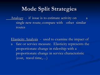
Mode Split Strategies • Analogy • Elasticity Analysis • Direct Estimation of Transit Share • Disaggregate Mode Split
Choosing a Mode Split Technique • Application • Time and budget constraints • Project costs • Existing data availability • Existing service? • if none, have to “borrow” a model
Selecting Analogy Routes • Selection based on similarities in: • Household characteristics • Transit service • Adjustments • Service area household characteristics • Service differences • Fare differences
Elasticities: ratio of change in demand over change in system
Example of Elasticity • If transit fares are raised from $1.00 to $1.25 and there is a resulting drop in daily transit ridership from 8,000 to 7,200, the elasticity, as calculated below, would be -0.40
Elasticity analysis example • What does the –0.4 factor mean? • typical values for cities range from -0.15 to -0.4 • Is this elastic, or inelastic? • Do you think larger cities would have larger or smaller elasticity? Why?
Direct Estimation of Transit Share • In small-to-medium regions with limited transit use • Particularly when transit use is limited to specific populations (zero-car household, students, and elderly) • Generally estimate district-to-district transit share • Find relationship between SE&D and %transit • Calibrate for base year • Assume relationship will hold in future • Subtract resulting transit trips from person trip table.
Disaggregate Mode Split Models • Travel is a result of choices • Elasticity, analogy, and direct estimation of transit share are limited, particularly in policy analysis • Output • Share of person trips using each mode (by trip purpose) for each production-attraction cell.
Disaggregate Mode Split Models Utility functions Building blocks for DMS models Rank desirability of the alternate transportation modes Deterministic equations Probability models (overcomes limitations of deterministic utility functions) Logit the most common Incorporate utility equations into probabilistic equations Binomial logit models Predict choice between two alternatives Multinomial logit models Predict choice between more than two alternatives
Disaggregate mode split using Utility Functions and Probabilistic Models • Input: Individual responses on mode desirability and usage to develop “Utility functions” • Preference and usage data may be from census or special home surveys. • System data such as travel time and cost generally from network data • usually don’t have the kind of data needed to know all users preferences
Observation v. prediction • If we wish to estimate transit by income level (or other detailed variable) in the future we need to be able to forecast the population characteristic in each group. • The more disaggregate the data set for modeling, the more difficult the prediction of future. Just like trip generation and distribution … can you give examples?
Binomial Logit Model Example Auto Utility Equation: UA= -0.025(IVT) -0.050(OVT) - 0.0024(COST) Transit Utility Equation: UB= -0.025(IVT) -0.050(OVT) – 0.10(WAIT) – 0.20(XFER) - 0.0024(COST) Where: IVT= in-vehicle time in minutes OVT = out of vehicle time in minutes COST = out of pocket cost in cents WAIT = wait time (time spent at bus stop waiting for bus) XFER = number of transfers Question: what is the implied cost of IVT? OVT? WAIT? XFER?
References • Transit Fact Book, 50th ed, American Public Transit Association, Washington, D.C. January 1999. • Federal Highway Administration. Traveler Response to Transportation System Changes. 2nd ed, U.S. Department of Transportation, Washington, D.C., July 1981. • Federal Transit Administration, A Self-Instructinf Course in Disaggregate Mode Choice Modeling. Report No. DOT-T-93-19. U.S. Department of Transportation, Washington, D.C., December 1986 • Meyer, M.D., and E.J. Miller. Urban Transportation Planning, A Decision-Oriented Approach. 2nd ed. McGraw-Hill, 2001.
Mode OVT IVT Cost (cents) 1 person 5 17 200.0 2-person carpool 5 21 100.0 3-person carpool 5 23 66.6 4-person carpool 5 25 50.0 Transit 7 33 160.0
Part 1: CALCULATE MODE PROBABILITIES BY MARKET SEGMENT • Overview: Calculate the mode probabilities for the trip interchanges. Use the tables on the next pages. • Part A: Calculate the utilities for transit as follows: • Insert in the table the appropriate values for OVT, IVT, and COST. • Calculate the utility relative to each variable by multiplying the variable by the coefficient which is shown in parenthesis at the top of the column; and • Sum the utilities (including the mode-specific constant) and put the total in the last column. • Part B: Calculate the mode probabilities as follows: • Insert the utility for transit in the first column; • Calculate eU for transit • Sum of eU for transit and put in the “Total” column; and • Calculate the probability for transit using the formula: • Sum the probabilities (they should equal 1.0)
Say, from trip distribution, the number of trips was 14,891. Calculate the number of trips by mode using the probabilities calculated. Mode Trips (Zone 5 to Zone 1)
If we had time … Source: publicpurpose.com
Cheaper to lease cars than provide new transit? http://www.publicpurpose.com/ut-2000rail.htm
Transit share dropping? http://www.publicpurpose.com/ut-intlmkt95.htm
Where rail transit works http://www.publicpurpose.com/utx-rails.htm
You can see an alternative view here: http://www.sprawlwatch.org/