Download
1 / 18
190 likes | 399 Views
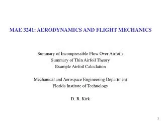
MAE 3241: AERODYNAMICS AND FLIGHT MECHANICS. Homework #4 Solution: Questions (1) – (4) Mechanical and Aerospace Engineering Department Florida Institute of Technology D. R. Kirk. QUESTION 1: SAMPLE MATLAB SCRIPT. close all; clear all; % Question 1 a=1; lambda=1;

E N D
MAE 3241: AERODYNAMICS ANDFLIGHT MECHANICS Homework #4 Solution: Questions (1) – (4) Mechanical and Aerospace Engineering Department Florida Institute of Technology D. R. Kirk
QUESTION 1: SAMPLE MATLAB SCRIPT close all; clear all; % Question 1 a=1; lambda=1; [x,y]=meshgrid(-5:0.01:5,-5:0.01:5); psi=lambda./2./pi.*atan(2.*x.*y./(x.^2-y.^2+a.^2)); % Now I am going to set some fixed values of the streamfunction psi to % plot. I am setting up a vector V which will range from the minimum value % of psi to the maximum value. I use the double command min(min(psi)) since % psi is two-dimensional, and the first min will find the minimum row and % the second the minimum of that row, or a single value. Same idea with % max(max(psi)). Since I wanted to plot 10+1 values of constant psi, I % arranged them to be equally spaced between the minimum and maximum value. V=[min(min(psi)):(max(max(psi))-min(min(psi)))/10:max(max(psi))]; cs=contour(x,y,psi,V); % Note the use of the contour function here. To use the streamline command we could have % found the the u and v components of the velocity, which would have added some complexity % to this problem. Since we are only interested in sketching some of the streamlines, % I simply plotted a constant values of psi without any regard for the exact values. % Note that this would involve iteration to solve the resulting equation for either x or y given % a constant value of psi. xlabel('x-direction'); ylabel('y-direction'); title('Homework #4: Question 1'); grid; % clabel(cs,V); % If you uncomment the above line, MATLAB will label all the contours for % you as well. It is a little messy so use the zooming tool to see what is % really going on, especially in Quesiton #2.
QUESTION 1: STREAMLINE PLOT • Find the stream function and plot some streamlines for the combination of a line source, L, at (x,y)=(0,a) and an equal line source located at (0,-a)
QUESTION 1: EXAMPLE OF LABELED CONTOURS • Find the stream function and plot some streamlines for the combination of a line source, L, at (x,y)=(0,a) and an equal line source located at (0,-a)
QUESTION 2: SAMPLE MATLAB SCRIPT % Question 2 gamma=-1; [x,y]=meshgrid(-2.001:0.01:2.001,-2:0.01:2); % Notice the choice on the starting and ending bounds that I have selected. % Since the natural log of 0 is negative infinity MATLAB has problems % plotting streamlines with this value. Therefore I selected some starting % and ending points that eliminate the argument of the natural log from % ever being zero. psi=gamma./2./pi.*log(sqrt((x-a).^2+y.^2))+gamma./2./pi.*log(sqrt((x+a).^2+y.^2)); figure(2) V=[min(min(psi)):(max(max(psi))-min(min(psi)))/20:max(max(psi))]; cs=contour(x,y,psi,V); clabel(cs,V); xlabel('x-direction'); ylabel('y-direction'); title('Homework #4: Question 2'); grid;
QUESTION 2: STREAMLINE PLOT • Find the stream function and plot some streamlines for the combination of a counterclockwise line vortex with strength G at (x,y)=(a,0) and an equal line vortex placed at (-a,0).
QUESTION 2: EXAMPLE OF LABELED CONTOURS • Find the stream function and plot some streamlines for the combination of a counterclockwise line vortex with strength G at (x,y)=(a,0) and an equal line vortex placed at (-a,0).
QUESTION 3: SAMPLE MATLAB SCRIPT, POLAR AND CARTESIAN % Question 3 in Polar Coordinates lambda=-1000; gamma=1600; [psi,r]=meshgrid(0:100:1000,0:0.01:10); theta=(psi-gamma./2./pi.*log(r))./(lambda./2./pi); % Note that here we were able to solve for theta explicitly, unlike either % x or y in Question (1) or Question (2). Also, I am not sure if MATLAB can % do contour plots in polar coordinates. figure(3) polar(theta,r); title('Homework #4: Question 3, Polar Approach'); grid; % Question 3 in Cartesian Coordinates lambda=-1000; gamma=1600; [x,y]=meshgrid(-10:0.1:10,-10:0.1:10); psi=lambda./2./pi.*atan(y./x)+gamma./2./pi.*log(sqrt(x.^2+y.^2)); figure(4) V=[min(min(psi)):(max(max(psi))-min(min(psi)))/20:max(max(psi))]; cs=contour(x,y,psi,V); xlabel('x-direction'); ylabel('y-direction'); title('Homework #4: Question 3, Cartesian Approach'); grid;
QUESTION 3: POLAR COORDINATES • A tornado is simulated by a line sink L=-1000 m2/s plus a line vortex G=1600 m2/s. Find the angle between any streamline and radial line, and show that it is independent of both r and q. If this tornado forms in sea-level standard air, what is the local pressure and velocity 25 meters from the center of the tornado?
QUESTION 3: CARTESIAN COORDINATES • A tornado is simulated by a line sink L=-1000 m2/s plus a line vortex G=1600 m2/s. Find the angle between any streamline and radial line, and show that it is independent of both r and q. If this tornado forms in sea-level standard air, what is the local pressure and velocity 25 meters from the center of the tornado? Explain what is going on here
QUESTION 3: INCREASED FIDELITY Why are these streamlines not continuous?
QUESTION 4: SAMPLE MATLAB SCRIPT % Question 4 close all; clear all; a=1; gamma=1; [x,y]=meshgrid(-3.001:0.01:3.001,-3:0.01:3); psi=-3.*gamma./2./pi.*log(sqrt(x.^2+(y-a).^2))+1.*gamma./2./pi.*log(sqrt(x.^2+(y+a).^2)); V=[min(min(psi)):(max(max(psi))-min(min(psi)))/50:max(max(psi))]; figure(1) contour(x,y,psi,V); xlabel('x-direction'); ylabel('y-direction'); title('Homework #4: Question 4'); grid; figure(2) phi=3.*gamma./2./pi.*atan((y-a)./x)-1.*gamma./2./pi.*atan((y+a)./x); Z=[min(min(phi)):(max(max(phi))-min(min(phi)))/50:max(max(phi))]; contour(x,y,psi,V); hold on; contour(x,y,phi,Z); xlabel('x-direction'); ylabel('y-direction'); title('Homework #4: Question 4'); grid;
QUESTION 1: FINDING MINIMUM VELOCITY USING SYMBOLIC MATH % find velocity components using MATLAB's symbolic toolbox syms x y a gamma u v psi=-3.*gamma./2./pi.*log(sqrt(x.^2+(y-1).^2))+1.*gamma./2./pi.*log(sqrt(x.^2+(y+1).^2)); % To find Velocity Components, take derivatives of psi with respect to x and y u=diff(psi,y); v=-diff(psi,x); % clear all a=1; gamma=1; [x,y]=meshgrid(-3:0.05:3,-3:0.05:3); u=-3./4.*gamma./pi./(x.^2+y.^2-2.*y+1).*(2.*y-2)+1./4.*gamma./pi./(x.^2+y.^2+2.*y+1).*(2.*y+2); v=3./2.*gamma./pi./(x.^2+y.^2-2.*y+1).*x-1./2.*gamma./pi./(x.^2+y.^2+2.*y+1).*x; V=sqrt(u.^2+v.^2); Vmin=min(min(V)) loc_Vmin=find(V==Vmin); xloc_Vmin=x(loc_Vmin); yloc_Vmin=y(loc_Vmin); % The following command will generate a 3-D picture of the velocity field figure(3) surf(x,y,V); hold on; plot3(xloc_Vmin,yloc_Vmin,Vmin,'.r','MarkerSize',20); colorbar; title('Homework #4: Question 4 Velocity Magnitude'); grid; xlabel('x-direction'); ylabel('y-direction'); zlabel('Velocity Magnitude'); % Examine velocity magnitude on constant x x=xloc_Vmin; y=-3:0.01:3; u=-3./4.*gamma./pi./(x.^2+y.^2-2.*y+1).*(2.*y-2)+1./4.*gamma./pi./(x.^2+y.^2+2.*y+1).*(2.*y+2); v=3./2.*gamma./pi./(x.^2+y.^2-2.*y+1).*x-1./2.*gamma./pi./(x.^2+y.^2+2.*y+1).*x; V=sqrt(u.^2+v.^2); figure(4) plot(y,V,yloc_Vmin,Vmin,'ro'); grid; legend('Velocity Magnitude on x=0','Location of Minimum Velocity','Location','NorthWest'); xlabel('y-direction'); ylabel('Magnitude of Velocity'); title('Plot of Velocity Profile between Vorticies');
QUESTION 4: PLOT OF y • A counterclockwise line vortex of strength 3G at (x,y)=(0,a) is combined with a clockwise vortex G at (0,-a). Plot the streamline and potential-line pattern, and find the point of minimum velocity between the two vorticies.