Solving First Order Ordinary Differential Equations with Matlab
300 likes | 900 Views
Solving First Order Ordinary Differential Equations with Matlab. Oct. 2, 2008. Example Problem. Consider an 80 kg paratrooper falling from 600 meters. The trooper is accelerated by gravity, but decelerated by drag on the parachute

Solving First Order Ordinary Differential Equations with Matlab
E N D
Presentation Transcript
Solving First Order Ordinary Differential Equations with Matlab Oct. 2, 2008
Example Problem • Consider an 80 kg paratrooper falling from 600 meters. • The trooper is accelerated by gravity, but decelerated by drag on the parachute • This problem is from Cleve Moler’s book called Numerical Computing with Matlab
Governing Equation • m= paratrooper mass (kg) • g= acceleration of gravity (m/s^2) • V=trooper velocity (m/s) • Initial velocity is assumed to be zero
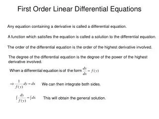
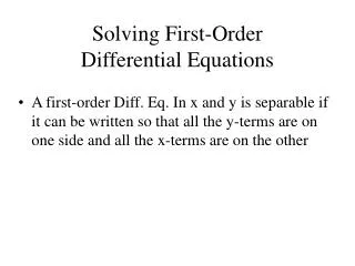
Preparing to Solve Numerically • First, we put the equation in the form • For our example, the equation becomes:
Solving Numerically • There are a variety of ODE solvers in Matlab • We will use the most common: ode45 • We must provide: • a function that defines the function derived on previous slide • Initial value for V • Time range over which solution should be sought
The Function function rk=f(t,y) mass=80; g=9.81; rk=-g+4/15*y^2/mass; Save as f.m The name of m.file has be saved as the same as the name of the function you define in this .m file.
The Solution clear all timerange=[0 30]; %seconds initialvelocity=0; %meters/second [t,y]=ode45(@f, timerange, initialvelocity) plot(t,y) xlabel(‘time(s)’) ylabel(‘velocity (m/s)’) Saved as example1.m
Options are available to: • Change relative or absolute error tolerances • Maximum number of steps • etc.