Survival analysis
How to analyze your organism’s chance of survival?. Survival analysis. Data in survival analysis. Data: Time between two distinct events, repeated among many subjects/objects/organisms. The first event is predefined while the second is typically some specific kind of transition .


Survival analysis
E N D
Presentation Transcript
How to analyze your organism’schance of survival? Survival analysis
Data in survival analysis Data: Time between two distinct events, repeated among many subjects/objects/organisms. The first event is predefined while the second is typically some specific kind of transition. The time between these two events will be called the transition time (or survival time) It can happen that subjects exit the study for other reasons than the event of interest. This is called censored data. Transition time is more than what we have registered, but we don’t know by how much. time
Examples of censoring events • Medical analysis – diagnosis to death by that disease: • End of the study • The patient wants to leave the study • Death by other causes • Plant survival study – start of experiment to death by environmental factors: • End of study • Experimenter accidentally dropped the pot on the ground • Start of larval stage until transition to adult: • End of the study • Death of the larva • Matriculation to master’s degree of students: • End of study • Student dropped out • Death of student (hopefully not!) If we disregard censored data, we can seriously underestimate the transition time!
Terminology • Subject: Whatsoever the start and end events belong to. • Transition: The end event. • Transition time: Time between the two events of interest. • Censoring: When a subject leave the study in a different way than the specified transition. • Age: Time from the start event to the present time for subjects which have not been censored and which have not undergone transition. • Treatment: Same as regression/dependent variable/explanation variable in ordinary regression. Finding the effect of a treatment on survival is typically the goal of survival analysis.
Concepts: transition time distribution The transition time will typically vary, so we need a statistical distribution for it. Distribution f(t) describes the probability-density of the transition times (t). A sharp peak around a value means most survival times are found around that value. A histogram of actual transition times will start to look like this distribution when we have much data. Distribution of age at death for the population of U.S.A. 2003, as derived from the histogram of ages.
Concepts: survival time distribution, survival curve and hazard Survival curve, S(t): Describes the probability of not going through a transition before a given age, t. A histogram of the age of subjects at a given time, will look like this curve. In more mathematical terms, it’s the cumulative sum (integral) of probabilities (densities) for all times larger than t. Survival curve for U.S.A. 2003, from the histogram of ages.
Concepts: survival time distribution, survival curve and hazard Hazard rate for U.S.A. 2003, derived from the histogram of ages. Hazard rate, h(t): The chance of going through a transition the next time interval, given that the subject has not done so earlier.
Concepts: survival time distribution, survival curve and hazard If we have an expression for one of these concepts, the other two can be derived. Just different ways of looking at the same thing.
Ex: Constant risk/hazard - the exponential distribution • Form: f(t)=e-t • Usage: • Unstable elementary particles • Radioactive isotopes • Time between phone calls • Life time of a particular copy of DNA for microbial organisms? PS: Conditioned on the state of the organism itself and it’s environment. • Special quality - memoryless: f(t-t0 | t>t0)=f(t) f(t)=e-t t0 Constant hazard. Reasonable, since the distribution is memoryless. S(t)=e-t If the survival probability drops to 50% in t=5, it will drop to 25% in t=10 and to 12.5% in t=15. h(t)=
Ex: The effects of genetic and env. variation – the Pareto distribution • Assume microbial survival is conditionally exponential distribution. • Contribution from genetics and environment spreads out the death rate, , according to the gamma distribution, (a,b). • Result: f(t)= (a/b) (1+t/b)-(a+1)(Pareto distribution) f(t) for a=1, b=1 h(t)=a/(b+t) • Dropping hazard rate. • Reasonable: • If old age => good genes and/or good env. • If young, over-representation of bad genes and/or bad env. S(t)=(1+t/b)-a
Ex: Aging – the uniform distribution • Cartoon model of aging: the uniform distribution: f(t)=I(0<t<a)/a • a=maximal age. • All outcomes below that are equally probable. f(t) Hazard rate increases inversely proportional to the distance to a. The closer to the maximum attainable age, the more risk there is of dying. S(t)=(1-t/a)I(0<t<a) h(t)=1/(a-t)
Ex: Hazard rate modeling – the bathtub curve • Often observed in engineering: a hazard rate that it higher for small and large times than for moderate times. • Can be reasonable for complex biological organisms also. For instance humans. • Possible to start with modeling hazard rates in order to make a transition time distribution. Estimated h(t) from census data 2003, U.S.A.
Increasing/decreasing hazard as seen from the survival curve • Increasing hazard survival-curve bends downwards on the log-scale. • Decreasing hazard survival-curve bends upwards on the log-scale. S(t) h(t) Example: Uniform transition time (cartoon of aging) S(t) h(t) Example: Pareto distribution (Varying genes/env. Possibly also a model for vulnerability in early life.)
Estimating the survival curve – the Kaplan-Meier estimator Kaplan-Meier is a parameter-free way of estimating the survival curve. • Similar to histograms, in that it simply summarizes the data. • Performed by first noting for which times, tj, there are transitions in the data. • The number of transitions, mj, and the number of subjects “at risk”, yj, (both subjects which will transit later and subjects that are later censored), is then used. • Technical: Example: Survival plot for plant experiment – all plants R code: survfit(Surv(t.event,censoring.status)) Use “plot”, to see the resulting curve.
Kaplan-Meier confidence intervals Divide your dataset into subgroups with different treatments and you get a feel for the difference between these treatments. (In this plant study, the treatment is day length, “dlen”): You can get a confidence interval for this estimated curve. R code: survfit(Surv(t.event,censoring.status)dlen, conf.type=“plain”, conf.int=0.95) PS: Note that using confidence intervals to say whether there is a difference means invoking a large number of dependent tests. Not ok. R code: survfit(Surv(t.event,censoring.status), conf.type=“plain”, conf.int=0.95)
Kaplan-Meier: The logrank test Does model comparison between grouping the data according to treatment and not grouping the data. Compares the observed number of events to that expected if the groups have equal transition time distribution. Gives a p-value for the zero-hypothesis (no effect of different treatments). R-code: survdiff(Surv(t.event,censoring)~treatment)
Cox regression • Addresses (almost all) the weaknesses of the Kaplan-Meier approach. • Does so by a single model assumption: proportional hazard. • Separates time dependency from variable dependency *in the hazard rate*. • Hazard ratio: The hazard rate for one choice of explanation variables divided by the hazard rate of another choice. • Allows for continuous explanation variables and additive effects of different categorical variables. • R-code: coxph(Surv(t.event,censoring)~var1+var2+var3)
Cox regression – interpretation of regression coefficients Proportional hazard regression: h(t|x)=h0(t)ex or lh(t|x)=lh0(t)+x where lh=log(h). Assume one explanation variable, x: What happens if we change it from x to x+1? • Log-hazard rate changes by a additive factor . • The hazard changes by a multiplicative factor e. • Log-survival curve also changes by a multiplicative factor e. (The latter can be compared to results from the Kaplan-Meier estimator.) • Survival curve changes from S(t) to S(t)exp(). (Ex: S(t|x=1)=S(t|x=0)2. Not so easy to see in a plot.) lh(t|x=1)= lh(t|x=0)+0.69 h(t|x=1)= 2h(t|x=0) log(S(t|x=1))= 2log(S(t|x=0))
Cox regression – model comparison • Gives a (partial) likelihood, so more model comparison techniques available. • Likelihood-ratio test • AIC/BIC • Wald test (comparison between estimate and standard error, implemented in R). • Stepwise adding/subtracting extra variables possible, either likelihood-based methods or by Wald test. • Full model exploration by information criteria also possible (though prohibitively costly when the number of explanation variables is high).
Cox regression – testing proportional hazard • Implemented in R: cox.zph(…) • What makes the hazard non-proportional can be viewer using the Kaplan-Meier-estimated log-survival-curve. (Or plot(cox.zph(…))) For this plant experiment, the survival-curves for short day length and long day length seem to part company at around day 30-40. Doesn’t necessarily invalidate the Cox-regression but makes the hazard ratio an average effect. Kaplan-Meier estimate for log-survival-curve