Behavior Modes
Behavior Modes. Meir Kalech Partially Based on slides of Brian Williams, Luca Console and Peter struss. Outline. Last lecture: Generation of tests/probes Measurement Selection Probabilities of Diagnoses Today’s lecture: Models of correct + faulty behavior Sherlock engine

Behavior Modes
E N D
Presentation Transcript
Behavior Modes Meir Kalech Partially Based on slides of Brian Williams, Luca Console and Peter struss
Outline • Last lecture: • Generation of tests/probes • Measurement Selection • Probabilities of Diagnoses • Today’s lecture: • Models of correct + faulty behavior • Sherlock engine • Abductive diagnosis • Qualitative models
Exploiting models of correct/faulty behavior Initial proposal: using only models of correct behavior • They are those that are in strict accordance with the goals (easy to acquire, e.g., from design) • But unfortunately they are not always sufficient • Need of exploiting also fault models of some form • predictive models [Struss, Dressler, 89] – GDE+[de Kleer, Williams 89] - SHERLOCK • “weak” models of physical impossibility [Friedrich et al. 90] • behavioral models [Console, Torasso, 91]
X Diagnosis With Only the Unknown Inverter(i): • G(i): Out(i) = not(In(i)) • U(i): A B C 0 0 0 Y • Isolates surprises • Doesn’t explain Nominal and Unknown Modes
X Diagnosis With Only the Known Inverter(i): • G(i): Out(i) = not(In(i)) • S1(i): Out(i) = 1 • S0(i): Out(i) = 0 A B C 0 0 0 Y • No surprises • Explains Exhaustive Fault Modes
X Solution: Diagnosis as Estimating Behavior Modes Inverter(i): • G(i): Out(i) = not(In(i)) • S1(i): Out(i) = 1 • S0(i): Out(i) = 0 • U(i): A B C 0 0 0 Y • Isolates surprises • Explains Nominal, Fault and Unknown Modes
Measurement motivation to use Behavior modes • Knowledge of failure modes is important to decide what measurement to make next. • If all faults were equally likely, measuring X or Y provides equal information. • Suppose: • Inverters A and B almost always fail by stuck-at-1. • Inverter C almost always fails by stuck at-0. • It is unlikely that inverter A is failing. • The likely failures of inverters B and C are consistent with the symptom
Behavior Modes • System comprises a (finite) set of components COMPS = { Ci } • Each Ci has a (finite) set of behavior modes modes(Ci) = { mij(Ci)} • E.g. • - (unique) correct behavior: ok(Ci) • - (any) faulty behavior: ok(Ci) • - a specific fault: stuck-closed(valvei) • Behavior mode operating mode (of correct behavior) • E.g. blocking mode of a diode • Definition (Mode Assignment) • COMPS’ COMPS • MA = {mij(Ci) Ci COMPS’ } • or MA = Ci COMPS’mij(Ci) • MA complete: COMPS’=COMPS
Diagnoses as Assignments of Fault Modes • Definition (Diagnosis): • A complete mode assignment MA that is consistent with the observations: • SDMA È OBS ^ • Definition (Mode Assignment) • COMPS’ COMPS • MA = {mij(Ci) Ci COMPS’ } • or MA = Ci COMPS’mij(Ci) • MA complete: COMPS’=COMPS
Battery Starter RLight HLight Yet Another Simple Example • Head lights work • Starter and rear light don’t • Obvious diagnosis: Starter and rear light are broken
Battery Starter RLight HLight Fault Localization for the Simple Example - Conflicts 1 and 2 • ok(Battery) ok(Wire1) ok(Wire2) ok(Starter) active(Starter) • OBS active(Starter) • Conflictok(Battery) ok(Wire1) ok(Wire2) ok(Starter) Wire1 Wire2 Wire3 Wire4 • Analogously: • ok(Battery)ok(Wire1) ok(Wire2)ok(Wire3) ok(Wire4) ok(RLight) Wire5 Wire6
Battery Starter RLight HLight Fault Localization for the Simple Example - Conflicts 3 and 4 • lit(HLight) ok(HLight) ok(Wire5) ok(Wire6) ok(RLight) lit(RLight) • OBS lit(RLight) • Conflictok(HLight) ok(Wire5) ok(Wire6) ok(RLight) Wire1 Wire2 Wire3 Wire4 • Analogously: • ok(HLight) ok(Wire5) ok(Wire6) ok(Wire3) ok(Wire4) ok(Starter) Wire5 Wire6
Battery Starter RLight HLight Fault Localization for the Simple Example - Hitting Sets • {Battery, Wire1, Wire2, Starter} • {Battery, Wire1, Wire2, Wire3, Wire4, Rlight} • {HLight, Wire5, Wire6, Rlight} • {Hlight, Wire5, Wire6, Wire3, Wire4, Starter} Wire1 Wire2 ? ! Wire3 Wire4 • {Starter, Rlight} • {Battery, HLight} Wire5 Wire6 • {Wire1, Wire5} • + 19 NONSENSES more!
Battery Starter • {Starter, Rlight} RLight • {Battery, HLight} • {Wire1, Wire5} HLight • + 19 more! What Makes Most of the Fault Localizations Implausible? • If the battery were broken, the headlights would not be lit • Broken headlights cannot be lit • Knowledge about faults can reduce the set of fault localizations Wire1 Wire2 ? ! Wire3 Wire4 Wire5 Wire6
Fault Models - “Physical Negation” • Fault models are needed • predictive: bulb(B) AB(B) voltageIn(B,X) light(B,off)
Outline • Last lecture: • Generation of tests/probes • Measurement Selection • Probabilities of Diagnoses • Today’s lecture: • Models of correct + faulty behavior • Sherlock engine • Abductive diagnosis • Qualitative models
Search Guided by Probabilities: SHERLOCK ([de Kleer- Williams 89]) • Basic Idea: Search for the most probable explanations of the observations • Fault models for each component (type) • Possible: unknown fault mode • Modes have prior probability • Mode assignments have a probability • SHERLOCK: best first search for consistent mode assignments • termination criteria
Leading Diagnoses • Complexity of diagnoses space: n-#components, m-#modesGDE 2n SHERLOCK: mn • To reduce the high complexity, generate only leading diagnoses: • Diagnoses are those with the highest probabilities. • No more than k1 (=5) leading diagnoses. • Candidates with probability less than 1/k2(=100) of the best diagnosis are not considered • The diagnoses need not include more than k3 (=0.75) of the total probability mass of the candidates.
0 A 1 B Model of Inverter X Mode Behavior Prior Ø X : Normal .99 Out = In N X : Stuck at 1 Out = 1 .006 1 X : Stuck at 0 Out = 0 .003 0 X : Unknown .001 U SHERLOCK - Example: Two Inverters
0 A 1 B Model of Inverter X Mode Behavior Prior Ø X : Normal .99 Out = In N X : Stuck at 1 Out = 1 .006 1 X : Stuck at 0 Out = 0 .003 0 X : Unknown .001 U SHERLOCK - Example: Two Inverters In slide 25 see how to generate conflicts and diagnoses • Conflicts: {AN,BN}, {B0}, {A1, BN}
0 A 1 B SHERLOCK - Example: Two Inverters • Conflicts: {AN,BN}, {B0}, {A1, BN} • Inspired by GDE + modes • Diagnosis is an explanation: SDMAOBS ┴ , where MA=CiCOMPSmij(Ci), (rather than a set of faulty components) • I.E., the diagnosis set contains all the combinations of the components’ modes except of conflicts.
0 A 1 B [[A , B ]] [[A , B ]] .00594 .00099 N 1 N U [[A , B ]] [[A , B ]] .00004 .00001 1 1 1 U [[A , B ]] [[A , B ]] [[A , B ]] .00297 .00002 .000003 0 N 0 1 0 U [[A , B ]] [[A , B ]] [[A , B ]] .00099 .00001 .000001 U N U 1 U U SHERLOCK - Example: Two Inverters Generated by ATMS Conflicts: {AN,BN}, {B0}, {A1, BN} Full diagnostic explanations with probabilities: Diagnoses set does not contain:{AN,BN}, {A1, BN}, and supersets of {B0}
0 A 1 B [[A , B ]] [[A , B ]] .00594 .00099 N 1 N U [[A , B ]] [[A , B ]] .00004 .00001 1 1 1 U [[A , B ]] [[A , B ]] [[A , B ]] .00297 .00002 .000003 0 N 0 1 0 U [[A , B ]] [[A , B ]] [[A , B ]] .00099 .00001 .000001 U N U 1 U U SHERLOCK - Example: Two Inverters Generated by ATMS Conflicts: {AN,BN}, {B0}, {A1, BN} Full diagnostic explanations with probabilities: • Exhaustive search impossible • Perform best first search
0 A 1 B Legend: x inconsistent SHERLOCK - Example: Search Strategy Generate the next explanation with the highest probability
A B C 0 0 1 X Y SHERLOCK, Process in details:1. Find Symptoms & Conflicts Conflict: not (G(A) and G(B) and G(C)) Finding conflict through ATMS, but generate focus environments G G 0 0 0 G 0 1
A B C 0 0 1 X Y More Symptoms & Conflicts not (S1(A) and G(B) and G(C) S1 G 0 0 0 G 0 1
A B C 0 0 X Y More Symptoms & Conflicts not (S0(B) and G(C)) S0 0 0 0 G 0 1
A B C 0 0 X Y More Symptoms & Conflicts not S1(C) S1 0 1 0
All Minimal Conflicts • < S1(C) > • < S0(B), G(C) > • < S1(A), G(B), G(C) > • < G(A), G(B), G(C) >
2. Constituent Diagnoses from Conflicts • Diagnosis is an explanation, so it must contains no conflict: • < S1(C) >: not S1(C):=> G(C) or S0(C) or U(C) • <S0(B) and G(C)>:not (S0(B) and G(C)) => not S0(B) or not G(C) => G(B) or S1(B) or U(B) or S1(C) or S0(C) or U(C) • < S1(A), G(B), G(C) >=> G(A),S0(A),U(A),S1(B),S0(B),U(B),S1(C),S0(C) or U(C) • < G(A), G(B), G(C) >=> S1(A),S0(A),U(A),S1(B),S0(B),U(B),S1(C),S0(C) or U(C)
3. Generating Kernel Diagnoses • [G(C),S0(C),U(C)] • [G(B),S1(B),U(B),S1(C),S0(C),U(C)] • [G(A),S0(A),U(A),S1(B),S0(B),U(B),S1(C),S0(C),U(C)] • [S1(A),S0(A),U(A),S1(B),S0(B),U(B),S1(C),S0(C),U(C)] • [U(C)]
3. Generating Kernel Diagnoses • [G(C),S0(C),U(C)] • [G(B),S1(B),U(B),S1(C),S0(C),U(C)] • [G(A),S0(A),U(A),S1(B),S0(B),U(B),S1(C),S0(C),U(C)] • [S1(A),S0(A),U(A),S1(B),S0(B),U(B),S1(C),S0(C),U(C)] • [U(C)] • [S0(C)]
3. Generating Kernel Diagnoses • [G(C),S0(C),U(C)] • [G(B),S1(B),U(B),S1(C),S0(C),U(C)] • [G(A),S0(A),U(A),S1(B),S0(B),U(B),S1(C),S0(C),U(C)] • [S1(A),S0(A),U(A),S1(B),S0(B),U(B),S1(C),S0(C),U(C)] • [U(C)] • [S0(C)] • [U(B),G(C)]
3. Generating Kernel Diagnoses • [G(C),S0(C),U(C)] • [G(B),S1(B),U(B),S1(C),S0(C),U(C)] • [G(A),S0(A),U(A),S1(B),S0(B),U(B),S1(C),S0(C),U(C)] • [S1(A),S0(A),U(A),S1(B),S0(B),U(B),S1(C),S0(C),U(C)] • [S1(B),G(C)] • [U(C)] • [S0(C)] • [U(B),G(C)]
3. Generating Kernel Diagnoses • [G(C),S0(C),U(C)] • [G(B),S1(B),U(B),S1(C),S0(C),U(C)] • [G(A),S0(A),U(A),S1(B),S0(B),U(B),S1(C),S0(C),U(C)] • [S1(A),S0(A),U(A),S1(B),S0(B),U(B),S1(C),S0(C),U(C)] • [S1(B),G(C)] • [U(A),G(B),G(C)] • [U(C)] • [S0(C)] • [U(B),G(C]
3. Generate Kernel Diagnoses • [G(C),S0(C),U(C)] • [G(B),S1(B),U(B),S1(C),S0(C),U(C)] • [G(A),S0(A),U(A),S1(B),S0(B),U(B),S1(C),S0(C),U(C)] • [S1(A),S0(A),U(A),S1(B),S0(B),U(B),S1(C),S0(C),U(C)] • [S1(B),G(C)] • [U(A),G(B),G(C)] • [S0(A),G(B),G(C)] • [U(C)] • [S0(C)] • [U(B),G(C] • These are the kernel diagnoses • But for [U(C)] (for instance), what are the modes of A and B? • The best first search finds the most likely modes of A and B.
No observations • With no observations Sherlock finds the single leading diagnosis • The unfocused Sherlock finds 43 diagnoses
Input I=0 • Sherlock computes the following environments: • The focused Sherlock finds no label for X=0 as it does not hold in the single leading diagnosis.
A B C 0 X Y
A B C 0 0 X Y • Suppose O=0 Minimal conflicts are: • < S1(C) > • < S0(B), G(C) > • < S1(A), G(B), G(C) > • < G(A), G(B), G(C) > • Leading candidates: Next highest probability: For instance: These are the most likely modes of A and B, beyond the kernel diagnosis U(C)
A B C 0 0 X Y • Now, the posterior behavior modes probabilities are: • ATMS labels are:
A B C 0 0 X Y Top 6 of 64 = 98.6% of P
Outline • Last lecture: • Generation of tests/probes • Measurement Selection • Probabilities of Diagnoses • Today’s lecture: • Models of correct + faulty behavior • Sherlock engine • Abductive diagnosis • Qualitative models
Abductive diagnosis • The definition above is based on consistency: • explanation consistent with the observations • Weak notion of explanation • A diagnosis D explains an observation m if it does not contradict m (D does not support not m). • Abductive diagnosis: • A stronger notion of explanation • Explanation implies the observations • A diagnosis D explains an observation m if it supports m (Dm). • Abductive diagnosis [Poole 87][Console, Torasso, 89]
Abductive diagnosis – Poole et al. 87 A different concept: • A diagnosis is not a logical consequence of our observations. Exactly the opposite: • The observation should be shown to be logical consequences of our knowledge and diagnosis.
Abductive diagnosis - definition Cxt: inputs. The data that let the diagnoser to make prediction about the behavior of the system • Given • SD • Modes • Observations, with the distinction between contextual data (Cxt) and observations (Obs) • Determine • An assignment of behavior modes to components D = {mi(ci) | mi Modes(ci) } • such that: • SD Cxt D |= Obs • (SD Cxt D consistent)
A continuum of definitionsConsole and Torasso 91 Given OBS, partition it into Obs1 Obs2 SD Cxt D Obs2 |= Obs1 SD Cxt D Obs1 Obs2 consistent Since Abduction diagnosis is more restrict than consistency:Abduction provides a subset of the solutions provided by consistency-based diagnosis Varying Obs1 we have a continuum of definitions: Obs1=OBS,Obs2= Ø abduction diagnosis of Poole86 Obs1=Ø, Obs2=OBS consistency based diagnosis
Abductive or Consistency? Criteria to select the most appropriate definition • abduction and consistency are the two extremes of a spectrum of alternatives • abduction is the most restrictive definition • it requires “complete” models • it provides a strong (physical) notion of explanation • consistency-based is less restrictive • less constraints on the models • weaker notion of explanation
Computing abductive diagnoses: an example oil_cup radiator Model: oil_cup(normal) oil_level(normal) oil_cup(holed) oil_loss(present) oil_loss(present) oil_below_car(present) oil_loss(present) oil_level(low) oil_level(normal) oil_gauge(normal) oil_level(low) oil_gauge(red) oil_level(normal) water_level(normal) engine(on) engine_temp(normal) ... normal holed normal holed oil_loss oil_level water_level oil_below_car normal low normal low oil_gauge water_temp normal red normal high engine_on Obs1 = {engine_temp(high)} Two minimal candidate explanations • E1 = { oil_cup(holed) } • E2 = {radiator(holed)} normal high engine_temp