Download
1 / 85
870 likes | 1.15k Views
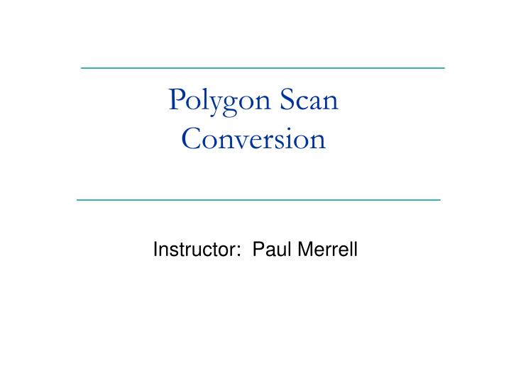
Polygon Scan Conversion. Instructor: Paul Merrell. Rasterization. Rasterization takes shapes like triangles and determines which pixels to fill. Filling Polygons. First approach: 1. Polygon Scan-Conversion

E N D
Polygon Scan Conversion Instructor: Paul Merrell
Rasterization Rasterization takes shapes like triangles and determines which pixels to fill.
Filling Polygons First approach: 1. Polygon Scan-Conversion Rasterize a polygon scan line by scan line, determining which pixels to fill on each line.
Filling Polygons Second Approach: Polygon Fill Select a pixel inside the polygon. Grow outward until the whole polygon is filled.
Why Polygons? You can approximate practically any surface if you have enough polygons. Graphics hardware is optimized for polygons (and especially triangles)
Coherence Scan-line Edge Span
Polygon Scan Conversion Intersection Points Other points in the span
Polygon Scan Conversion Process each scan line Find the intersections of the scan line with all polygon edges. Sort the intersections by x coordinate. Fill in pixels between pairs of intersections using an odd-parity rule. Set parity even initially. Each intersection flips the parity. Draw when parity is odd.
Polygon Scan-Conversion Process for scan converting polygons Process one polygon at a time. Store information about every polygon edge. Compute spans for each scan line. Draw the pixels between the spans. This can be optimized using an table that stores information about each edge. Perform scan conversion one scan line at a time.
Computing Intersections For each scan line, we need to know if it intersects the polygon edges. It is expensive to compute a complete line-line intersection computation for each scan line. After computing the intersection between a scan line and an edge, we can use that information in the next scan line.
Scan Line Intersection Polygon Edges Intersection points needed Previous scan line yi Current scan line yi+1 Intersection points from previous scan line
Scan Line Intersection Use edge coherence to incrementally update the x intersections. We know Each new scan line is 1 greater in y We need to compute x for a given scan line, (x@ymax,ymax) (x@ymin,ymin)
Scan Line Intersection So, and then This is a more efficient way to compute xi+1.
Edge Tables • We will use two different edge tables: • Active Edge Table (AET) • Stores all edges that intersect the current scan line. • Global Edge Table (GET) • Stores all polygon edges. • Used to update the AET.
Active Edge Table Table contains one entry per edge intersected by the current scan line. At each new scan line: Compute new intersections for all edges using the formula. Add any new edges intersected. Remove any edges no longer intersected. To efficiently update the AET, we will can use a global edge table (GET)
Global Edge Table Example D 8 7 C 6 5 B E 4 3 2 1 A 0 0 1 2 3 4 5 6 7 8 Place entries into the GET based on the ymin values. GET 8 (ymax, x@ymin, 1/m) 7 8, 6, -3/2 6 CD Indexed by scan line 6, 3, 3 5 BC 8, 0, ¾ 4 DE 3 AB = (2, 1), (3, 5) BC = (3, 5), (6, 6) CD = (6, 6), (3, 8) DE = (3, 8), (0, 4) EA = (0, 4), (2, 1) 2 AB EA 5, 2, ¼ 4, 2, -2/3 1 0
Active Edge Table Example The active edge table stores information about the edges that intersect the current scan line. Entries are The ymax value of the edge The x value where the edge intersects the current scan line. The x increment value (1/m) Entries are sorted by x values.
Active Edge Table Example D 8 7 C 6 5 B E 4 3 2 1 A 0 0 1 2 3 4 5 6 7 8 The ymax value for that edge The x value where the scan line intersects the edge. The x increment value (1/m) (ymax, x, 1/m) AET Scan Line 3 4, 2/3, -2/3 5, 5/2, 1/4 EA AB AB = (2, 1), (3, 5) BC = (3, 5), (6, 6) CD = (6, 6), (3, 8) DE = (3, 8), (0, 4) EA = (0, 4), (2, 1)
Active Edge Table Example D 8 7 C 6 5 B E 4 3 2 1 A 0 0 1 2 3 4 5 6 7 8 The ymax value for that edge The x value where the scan line intersects the edge. The x increment value (1/m) (ymax, x, 1/m) AET Scan Line 4 4, 2/3, -2/3 8, 0, 3/4 5, 11/4, 1/4 5, 5/2, 1/4 EA DE AB Scan Line 4 In the GET, edge DE is stored in bucket 4, so it gets added to the AET. ymax = 4 for EA, so it gets removed from the AET. New x value for AB is 5/2 + 1/4 = 11/4 AB = (2, 1), (3, 5) BC = (3, 5), (6, 6) CD = (6, 6), (3, 8) DE = (3, 8), (0, 4) EA = (0, 4), (2, 1)
Active Edge Table Example D 8 7 C 6 5 B E 4 3 2 1 A 0 0 1 2 3 4 5 6 7 8 The ymax value for that edge The x value where the scan line intersects the edge. The x increment value (1/m) Scan Line 5 (ymax, x, 1/m) AET 8, 3/4, 3/4 8, 0, 3/4 5, 11/4, 1/4 6, 3, 3 DE AB BC Increment x = 0 + 3/4 Remove AB, since ymax = 5. Add BC since it is in the GET at ymin = 5. AB = (2, 1), (3, 5) BC = (3, 5), (6, 6) CD = (6, 6), (3, 8) DE = (3, 8), (0, 4) EA = (0, 4), (2, 1)
Active Edge Table Example D 8 7 C 6 Scan Line 6 5 B E 4 3 2 1 A 0 0 1 2 3 4 5 6 7 8 AB = (2, 1), (3, 5) BC = (3, 5), (6, 6) CD = (6, 6), (3, 8) DE = (3, 8), (0, 4) EA = (0, 4), (2, 1)
Line Clipping What happens when one or both endpoints of a line segment are not inside the specified drawing area? Drawing Area
Line Clipping Strategies for clipping: Check (in inner loop) if each point is inside Works, but slow Find intersection of line with boundary Correct if (x ≥ xmin and x ≤ xmax and y ≥ ymin and y ≤ ymax) drawPoint(x,y,c); Clip line to intersection
Line Clipping: Possible Configurations Both endpoints are inside the region (line AB) No clipping necessary One endpoint in, one out (line CD) Clip at intersection point Both endpoints outside the region: No intersection (lines EF, GH) Line intersects the region (line IJ) Clip line at both intersection points J D I A F C H B E G
Line Clipping: Cohen-Sutherland Basic algorithm: Accept lines that have both endpoints inside the region. J D I Clip and retest A F C H B Trivially accept E G Trivially reject • Reject lines that have both endpoints less than xmin or ymin or greater than xmax or ymax. • Clip the remaining lines at a region boundary and repeat the previous steps on the clipped line segments.
Cohen-Sutherland: Accept/Reject Tests Assign a 4-bit code to each endpoint c0, c1based on its position: 1st bit (1000): if y > ymax 2nd bit (0100): if y < ymin 3rd bit (0010): if x > xmax 4th bit (0001): if x < xmin Test using bitwise functions if c0 | c1 = 0000 accept (draw) else if c0 & c1 0000 reject (don’t draw) else clip and retest 1001 1000 1010 0001 0000 0010 0101 0100 0110
Cohen-Sutherland Accept/Reject 1001 1000 1010 0001 0000 0010 0101 0100 0110 Accept/reject/redo all based on bit-wise Boolean ops.
Polygon Clipping What about polygons?
Polygon Clipping: Example p0 Line intersect boundary: Yes v6 v7 Clip first to ymin and ymax v0 v8 vertex:v0 ymax Inside region: No v9 v5 v1 v2 Add p0 to output list ymin v3 v4 Input vertex list:(v0, v1, v2, v3, v4, v5, v6, v7, v8, v9) Output vertex list: p0
Polygon Clipping: Example p0 line intersect boundary: no v6 v7 Clip first to ymin and ymax v0 v8 vertex:v1 ymax inside region: yes v9 v5 v1 v2 add v1 to output list ymin v3 v4 Input vertex list:(v0, v1, v2, v3, v4, v5, v6, v7, v8, v9) Output vertex list: p0 , v1
Polygon Clipping: Example p0 line intersect boundary: yes p1 v6 v7 Clip first to ymin and ymax v0 v8 vertex:v2 ymax inside region: yes v9 v5 v1 v2 add v2, p1 to output list ymin v3 v4 Input vertex list:(v0, v1, v2, v3, v4, v5, v6, v7, v8, v9) Output vertex list: p0 ,v1 , v2, p1
Polygon Clipping: Example p0 line intersect boundary: no p1 v6 v7 Clip first to ymin and ymax v0 v8 vertex:v3 ymax inside region: no v9 v5 v1 v2 ymin v3 v4 Input vertex list:(v0, v1, v2, v3, v4, v5, v6, v7, v8, v9) Output vertex list: p0, v1, v2, p1
Polygon Clipping: Example p0 line intersect boundary: yes p1 p2 v6 v7 Clip first to ymin and ymax v0 v8 vertex:v4 ymax inside region: no v9 v5 v1 v2 add p2 to output list ymin v3 v4 Input vertex list:(v0, v1, v2, v3, v4, v5, v6, v7, v8, v9) Output vertex list: p0, v1, v2, p1 , p2
Polygon Clipping: Example p3 p0 line intersect boundary: yes p1 p2 v6 v7 Clip first to ymin and ymax v0 v8 vertex:v5 ymax inside region: yes v9 v5 v1 v2 add v5, p3 to output list ymin v3 v4 Input vertex list:(v0, v1, v2, v3, v4, v5, v6, v7, v8, v9) Output vertex list: p0, v1, v2, p1, p2 , v5, p3
Polygon Clipping: Example p3 p0 line intersect boundary: no p1 p2 v6 v7 Clip first to ymin and ymax v0 v8 vertex:v6 ymax inside region: no v9 v5 v1 v2 ymin v3 v4 Input vertex list:(v0, v1, v2, v3, v4, v5, v6, v7, v8, v9) Output vertex list: p0, v1, v2, p1, p2, v5, p3
Polygon Clipping: Example p3 p0 line intersect boundary: no p1 p2 v6 v7 Clip first to ymin and ymax v0 v8 vertex:v7 ymax inside region: no v9 v5 v1 v2 ymin v3 v4 Input vertex list:(v0, v1, v2, v3, v4, v5, v6, v7, v8, v9) Output vertex list: p0, v1, v2, p1, p2, v5, p3
Polygon Clipping: Example p4 p3 p0 line intersect boundary: yes p1 p2 v6 v7 Clip first to ymin and ymax v0 v8 vertex:v8 ymax inside region: no v9 v5 v1 v2 add p4 to output list ymin v3 v4 Input vertex list:(v0, v1, v2, v3, v4, v5, v6, v7, v8, v9) Output vertex list: p0, v1, v2, p1, p2, v5, p3 , p4
Polygon Clipping: Example p4 p3 p5 p0 line intersect boundary: yes p1 p2 v6 v7 Clip first to ymin and ymax v0 v8 vertex:v9 ymax inside region: yes v9 v5 v1 v2 add v9, p5 to output list ymin v3 v4 Input vertex list:(v0, v1, v2, v3, v4, v5, v6, v7, v8, v9) Output vertex list: p0, v1, v2, p1, p2, v5, p3, p4 , v9, p5
Polygon Clipping: Example p4 p3 p5 p0 p1 p2 This gives us a new polygon ymax v9 v5 v1 v2 ymin with vertices: (p0, v1, v2, p1, p2, v5, p3, p4, v9, p5)
Polygon Clipping: Example (cont.) p4 p3 p5 p0 p1 p2 Now clip to xmin and xmax xmin xmax p9 v9 p6 v5 p7 v1 v2 p8 Input vertex list:= (p0, v1, v2, p1, p2, v5, p3, p4, v9, p5) Output vertex list:(p0, p6, p7, v2, p1, p8, p9, p3, p4, v9, p5)
Polygon Clipping: Example (cont.) Now post-process xmin xmax p4 p3 p5 p0 p9 v9 p6 p7 v2 p1 v3 p8 Output vertex list:(p0, p6, p7, v2, p1, p8, p9, p3, p4, v9, p5) Post-process:(p0, p6, p9, p3,) and (p7, v2, p1, p8) and (v4, v9, p5)
General Transformations Want to be able to manipulate graphical objects: Translation: move an object Rotation: change orientation Scale: change size Other transformations: reflection, shear, etc. A general 2-D transformation has the form: x´ = fx(x, y) y´ = fy(x, y) where x and y are the original coordinates and x´ and y´ are the transformed coordinates. In vector form:
General Transformations (cont.) General transforms may be non-linear: Lines do not necessarily map to lines Every point (along lines, inside shapes, etc.) needs to be transformed Non-linear Transformations are harder to deal with. Fortunately, many important transformations are linear. Non-Linear Example: y y 7 7 6 6 5 5 4 4 3 3 2 2 1 1 x x 0 0 0 0 1 1 2 2 3 3 4 4 5 5 6 6 7 7
Linear Transformations We will use linear transformations: x´ = fx(x, y) = axx + bxy + cx y´ = fy(x, y) = ayx + byy + cy Linear Transforms can be written using matrix operations: Advantages: Lines transform to lines Only need to transform vertices. Computationally efficient Problem: would like to simplify further get rid of T
Translation Move object from one place to another: Forward transform: x´ = x + tx y´ = y + ty or p´ = p + T where Inverse transform: p = p´ – T y 7 6 5 4 3 2 1 x 0 0 1 2 3 4 5 6 7
Scale Change an object’s size: Forward transform: x´ = sxx y´ = syy or p´ = Sp where Inverse transform: p = S-1p´ where y 7 6 5 4 3 2 1 x 0 0 1 2 3 4 5 6 7 Why do we get an apparent translation?
Scale Properties of the scale: The scale is performed relative to the origin. A scale factor greater than one enlarges the objects and moves it away from the origin. A scale factor less than one shrinks the object and moves it towards the origin. Usually this isn’t what we want Generally we would like to scale about the object’s center - not the coordinate origin.
Scale can accomplish the following transforms: Uniform scale: sx = sy Preserves angles, but not lengths Non-uniform scale: sxsy Doesn’t preserve angles or lengths Reflection about the x-axis:sx = 1, sy = –1 y-axis:sx = –1, sy = 1 line y = –x:sx = –1, sy = –1 Reflection preserves angles and lengths What is the inverse matrix? A reflection matrix is its own inverse. Scale: Transforms y 7 6 5 4 3 2 1 x 0 0 1 2 3 4 5 6 7 y = –x