Statistical Estimation Techniques: Confidence Intervals and Sample Size Calculations
This chapter delves into statistical inference tools such as estimation and hypothesis testing. Explore examples of one-sample estimation techniques, including confidence intervals for unknown parameters. Learn to calculate sample sizes and interpret confidence intervals. Discover estimation methods when the variance is unknown and understand how to determine confidence intervals in such scenarios. Gain insights into tolerance limits, prediction intervals, and estimating differences between two means. Expand your knowledge of statistical estimation techniques in this comprehensive guide.

Statistical Estimation Techniques: Confidence Intervals and Sample Size Calculations
E N D
Presentation Transcript
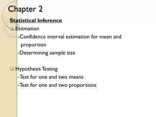
Chapter 9: One- and Two- Sample Estimation • Statistical Inference • Estimation • Tests of hypotheses • “Even the most efficient unbiased estimator is unlikely to estimate the population parameter exactly.” (Walpole et al, pg. 272) • Interval estimation: (1 – α)100% confidence interval for the unknown parameter. • Example: if α = 0.01, we develop a _______ confidence interval.
Single Sample: Estimating the Mean • Given: • σ is known and X is the mean of a random sample of size n, • Then, • the (1 – α)100% confidence interval for μ is given by
Example A traffic engineer is concerned about the delays at an intersection near a local school. The intersection is equipped with a fully actuated (“demand”) traffic light and there have been complaints that traffic on the main street is subject to unacceptable delays. To develop a benchmark, the traffic engineer randomly samples 25 stop times (in seconds) on a weekend day. The average of these times is found to be 13.2 seconds, and the variance is known to be 4 seconds2. Based on this data, what is the 95% confidence interval (C.I.) around the mean stop time during a weekend day?
Example (cont.) X = ______________ σ = _______________ α = ________________ α/2 = _____________ Z0.025 = _____________ Z0.975 = ____________ __________________ < μ < ___________________
Your turn … • What is the 90% C.I.? What does it mean?
How big a sample do we need? • If we want to be sure that our error in estimating µ is less than a specified amount, e, the required sample size is given by, • In our example, if the traffic engineer wants to be 95% confident that the mean stop time is off by less than 0.1, then he should take n = ___________________________________ samples. EGR 252 - Ch. 9 6
What if σ2is unknown? For example, what if the traffic engineer doesn’t know the variance of this population? • If n is sufficiently large (> _______), then the large sample confidence interval is: • Otherwise, must use the t-statistic …
Single Sample: Estimating the Mean(σ unknown, n not large) • Given: • σ is unknown and X is the mean of a random sample of size n (where n is not large), • Then, • the (1 – α)100% confidence interval for μ is given by
Recall Our Example A traffic engineer is concerned about the delays at an intersection near a local school. The intersection is equipped with a fully actuated (“demand”) traffic light and there have been complaints that traffic on the main street is subject to unacceptable delays. To develop a benchmark, the traffic engineer randomly samples 25 stop times (in seconds) on a weekend day. The average of these times is found to be 13.2 seconds, and the sample variance, s2, is found to be 4 seconds2. Based on this data, what is the 95% confidence interval (C.I.) around the mean stop time during a weekend day?
Example (cont.) X = ______________ s = _______________ α = ________________ α/2 = _____________ t0.025,24 = _____________ __________________ < μ < ___________________
Your turn A thermodynamics professor gave a physics pretest to a random sample of 15 students who enrolled in his course at a large state university. The sample mean was found to be 59.81 and the sample standard deviation was 4.94. Find a 99% confidence interval for the mean on this pretest.
Solution X = ______________ s = _______________ α = ________________ α/2 = _____________ (draw the picture) T___ , ____ = _____________ __________________ < μ < ___________________
Standard Error of a Point Estimate • Case 1: σ known • The standard deviation, or standard error of X is • Case 2: σ unknown, sampling from a normal distribution • The standard deviation, or (usually) estimated standard error of X is ______
9.6: Prediction Interval • For a normal distribution of unknown mean μ, and standard deviation σ, a 100(1-α)% prediction interval of a future observation, x0is if σ is known, and if σ is unknown
9.7: Tolerance Limits • For a normal distribution of unknown mean μ, and unknown standard deviation σ, tolerance limits are given by x + ks where k is determined so that one can assert with 100(1-γ)% confidence that the given limits contain at least the proportion 1-α of the measurements. • Table A.7 gives values of k for (1-α) = 0.9, 0.95, 0.99; γ = 0.05, 0.01; and for selected values of n.
Summary • Confidence interval population mean μ • Prediction interval a new observation x0 • Tolerance interval a (1-α) proportion of the measurements can be estimated with a 100(1-γ)% confidence
Estimating the Difference Between Two Means • Given two independent random samples, a point estimate the difference between μ1 and μ2 is given by the statistic We can build a confidence interval for μ1 - μ2 (given σ12 and σ22 known) as follows:
An example • Look at example 9.9, pg. 289
Differences Between Two Means: Variances Unknown • Case 1: σ12 and σ22 unknown but equal Where,
Differences Between Two Means: Variances Unknown • Case 2: σ12 and σ22 unknown and not equal Where,
Estimating μ1 – μ2 • Example (σ12 and σ22 known) : A farm equipment manufacturer wants to compare the average daily downtime of two sheet-metal stamping machines located in two different factories. Investigation of company records for 100 randomly selected days on each of the two machines gave the following results: x1 = 12 minutes x2 = 10 minutes 12 = 12 22 = 8 n1 = n2 = 100 Construct a 95% C.I. for μ1 – μ2
Solution Picture α/2 = _____________ z_____ = ____________ __________________ < μ1 – μ2 < _________________ Interpretation:
μ1 – μ2 : σi2 Unknown • Example (σ12 and σ22 unknown but equal): Suppose the farm equipment manufacturer was unable to gather data for 100 days. Using the data they were able to gather, they would still like to compare the downtime for the two machines. The data they gathered is as follows: x1 = 12 minutes x2 = 10 minutes s12 = 12 s22 = 8 n1 = 18 n2 = 14 Construct a 95% C.I. for μ1 – μ2
Solution Picture α/2 = _____________ t____ , ________= ____________ __________________ < μ1 – μ2 < _________________ Interpretation:
Paired Observations • Suppose we are evaluating observations that are not independent … For example, suppose a teacher wants to compare results of a pretest and posttest administered to the same group of students. • Paired-observation or Paired-sample test … Example: murder rates in two consecutive years for several US cities (see attached.) Construct a 90% confidence interval around the difference in consecutive years.
Solution Picture D = ____________ tα/2, n-1 = _____________ a (1-α)100% CI for μ1 – μ2 is: __________________ < μ1 – μ2 < _________________ Interpretation:
C.I. for Proportions • The proportion, P, in a binomial experiment may be estimated by where X is the number of successes in n trials. • For a sample, the point estimate of the parameter is • The mean for the sample proportion is and the sample variance
C.I. for Proportions • An approximate (1-α)100% confidence interval for p is: • Large-sample C.I. for p1 – p2is: Interpretation: _______________________________
Example 9.16 • C.I. = (-0.0017, 0.0217), therefore no reason to believe there is a significant decrease in the proportion defectives using the new process. • What if the interval were (+0.0017, 0.0217)? • What if the interval were (-0.9, -0.7)?