Download
1 / 38
390 likes | 534 Views
Orthogonal Range Searching I. Range Trees. Range Searching. S = set of geometric objects Q = query object Report/Count objects in S that intersect Q. Query Q. Report/Count answers. Single-shot Vs Repeatitive. Query may be: Single-shot (one-time). No need to preprocess

E N D
Orthogonal Range Searching I Range Trees
Range Searching • S = set of geometric objects • Q = query object • Report/Count objects in S that intersect Q Query Q Report/Count answers
Single-shot Vs Repeatitive • Query may be: • Single-shot(one-time). No need to preprocess • Repeatitive-Mode. Many queries are expected. Preprocess S into a Data Structure so that queries can be answered fast
Efficiency Measures • Repetitive-Mode • Preprocessing Time: P(n) • Space occupied by Data Structure: S(n) • Query Time: Q(n) • Dynamic Case: Update Time U(n) • Single-Shot • Space S(n) and Time T(n)
Orthogonal Range Searching in 1D • S: Set of points on real line. • Q= Query Interval [a,b] b a Which query points lie inside the interval [a,b]?
Orthogonal Range Searching in 2D • S = Set of points in the plane • Q = Query Rectangle
Binary search trees A binary search tree (BST) is a binary tree which has the following properties: • Each node has a value. • A total order is defined on these values. • The left subtree of a node contains only values less than the node's value. • The right subtree of a node contains only values greater than or equal to the node's value. The major advantage of binary search trees is that the related sorting algorithms and search algorithms such as in-order traversal can be very efficient.
6 17 1D Range Query Build a balanced search tree where all data points are stored in the leaves . 2 4 5 7 8 12 15 19 7 query: O(log n+k) 4 12 space: O(n) 2 5 8 15 2 4 5 7 8 12 15 19
Querying Strategy • Given interval [a,b], search for a and b • Find where the paths split, look at subtrees inbetween Paths split a b Problem: linking leaves do not extends to higher dimensions. Idea: if parents knew all descendants, wouldn’t need to link leaves.
Efficiency • Preprocessing Time: O(n log n) • Space: O(n) • Query Time: O(log n + k) • k = number of points reported • Output-sensitive query time • Binary search tree can be kept balanced in O(log n) time per update in dynamic case
1D Range Counting • S = Set of points on real line • Q= Query Interval [a,b] • Count points in [a,b] Solution: At each node, store count of number of points in the subtree rooted at the node. Query: Similar to reporting but add up counts instead of reporting points. • Query Time: O(log n)
y y2 y1 x x1 x2 2D Range queries • How do you efficiently find points that are inside of a rectangle? • Orthogonal range query ([x1, x2], [y1,y2]): find all points (x, y) such that x1<x<x2 and y1<y<y2
BST on y-coords Ty(v) T v P(v) P(v) BST on x-coords Range trees • Canonical subsetP(v) of a node v in a BST is a set of points (leaves) stored in a subtree rooted at v • Range tree is a multi-level data structure: • The main tree is a BST T on the x-coordinate of points • Any node v of T stores a pointer to a BST Ty(v) (associated structure of v), which stores canonical subset P(v) organized on the y-coordinate • 2D points are stored in all leaves!
For each internal node vTx let P(v) be set of points stored in leaves of subtree rooted at v. Set P(v) is stored with v as another balanced binary search tree Ty(v) (descendants by y) on y-coordinate. (have pointer from v to Ty(v)) Range trees Tx Ty(v) T4 p5 p4 p3 p2 p6 p1 p7 Ty(v) v v p7 p5 p6 p1 p2 p3 p4 p5 p6 p7 P(v) P(v) 14
The diagram below shows what is stored at one node. Show what is stored at EVERY node. Note that data is only stored at the leaves. Range trees Tx Ty(v) T4 p5 p4 p3 p2 p6 p1 p7 Ty(v) v v p7 p5 p6 p1 p2 p3 p4 p5 p6 p7 P(v) P(v) 15
Query: [x,x’] x’ x Range trees The query time: Querying a 1D-tree requires O(log n+k) time. How many 1D trees (associated structures) do we need to query? At most 2 height of T = 2 log n Each 1D query requires O(log n+k’) time. Query time = O(log2 n + k) Answer to query = Union of answers to subqueries: k = ∑k’.
Size of the range tree • Size of the range tree: • At each level of the main tree associated structures store all the data points once (with constant overhead): O(n). • There are O(log n) levels. • Thus, the total size is O(n log n).
Building the range tree • Efficient building of the range tree: • Sort the points on x and on y (two arrays: X,Y). • Take the median v of X and create a root, build its associated structure using Y. • Split X into sorted XL and XR, split Y into sorted YL and YR (s.t. for any pÎXL or pÎYL, p.x < v.x and for any pÎXR or pÎYR, p.x ³ v.x). • Build recursively the left child from XL and YL and the right child from XR and YR. • The running time isO(n log n).
Generalizing to higher dimensions • d-dimensional Range Tree can be build recursively from (d-1) dimensional range trees. • Build a Binary Search Tree on coordinates for dimension d. • Build Secondary Data Structures with (d-1) dimensional Range Trees. • Space O(n logd-1 n). • Query Time O(logd n + k).
Fractional Cascading • Search on a subset can be speeded up by adding pointers 10 19 23 33 38 42 55 66 68 3 19 33 42 55 68 10
Layered Range Trees • Node v and subtrees Left(v) and Right(v). • Secondary Structures T(Left(v)) and T(Right(v)) are built on subsets of points on which secondary structure T(v) is built. • Fractional Cascading can be used to speed up searches. • d-dimensional (d >= 2) Range Tree with fractional cascading: • Space: O(n logd-1n) • Query Time: O(logd-1 n + k)
Range trees: summary • Range trees • Building (preprocessing time): O(n log n) • Size: O(n log n) • Range queries: O(log2n + k) • Running time can be improved to O(log n + k) without sacrificing the preprocessing time or size: • Layered range trees (uses fractional cascading)
Application • Given a set of rectangles, report all pairs of rectangles (R1,R2) such that R1 encloses R2 d y2 y1 c a x1 x2 b
Reduction to Range Search • x1 >= a, x2 <= b, y1 >= c, y2 <= d. • x1 ε [a, infty], x2 ε [-infty,b], • y1 ε [c, infty], y2 ε [-infty,d]. • This is a 4D Range Search Problem: • Map each rectangle to 4D point and create a data structure D. • Map each rectangle to 4D interval and query D. • O(n log3 n) space and O(log4 n + k) query time, but O(log3 n + k) query time using fractional cascading.
Orthogonal Range Searching II Interval Trees
1D point enclosure S : set of n intervals on the real line. q : query point. Query: Which intervals contain Q? Build a data structure with the intervals, so that queries can be answered fast.
Subdivide the problem • Consider all 2n endpoints. • Xmid = Median of the endpoints. • At most half the midpoints are to the left of the median, at most half to the right. • Construct a binary tree based on this idea with Xmidas the “root discriminator”.
Subdivide set of intervals What do we do with the segments that intersect xmid? Imid Ileft Iright xmid
xmid Imid Interval trees Idea: Use an associated data structure! xmid
xmid L L Interval trees Idea: Store the segments twice; once for the left endpoints and once for the right endpoints. Need sorted list of left and right endpoints Sorted list of left endpoints
Recursive subdivision Left and right subtrees are interval trees. The interval tree has O(log n) depth and uses O(n) storage (each interval gets stored exactly at one node).
Querying If q < Xmid • consider left endpoints in Imid • query left subtree recursively Else • consider right endpoints in Imid • query right subtree recursively
Efficiency • Preprocessing Time O(n log n). • Space O(n). • Query Time = O(log n + k) : • we visit at most one node at any depth of the tree. • we report kv intervals at node v. • k = total number of intervals reported, k = ∑kv.
Application S: set of horizontal line segments in the plane. q: vertical line segment. Query: find all horizontal segments intersecting q. q
Solution • Build Interval Tree on Horizontal Segments. • Instead of storing left and right endpoints in an ordered list we need a secondary data structure at each node. Secondary data structure = 2D range tree
Analysis • Secondary data structure = 2D range tree: • O(n log n) space. • O(log n + k’) query time. • Overall: • Preprocessing Time: O(n log n). • Space: O(n log n) (we have range trees instead of ordered lists). • At each of the O(log n) nodes v on the search path we spend O(log n + kv) time. • Overall Query Time: O(log2 n + k). k = total number of intervals reported, k = ∑kv.
Windowing Query S: axes parallel segments. q: query axes parallel rectangle. Query: find all horizontal segments intersecting q.
Solution • Can be solved with range trees and interval trees. • Consider 2 subproblems: • Intervals with some endpoint in query. Range trees: • O(log n + k’) query time • O(n log n) space and preprocessing • Number of endpoints inside query. Interval trees: • O(log2 n + k’’) query time • O(n log n) space and preprocessing • Overall: • Preprocessing Time: O(n log n). • Query Time O(log2 n + k). • Space O(n log n).