Download
1 / 93
930 likes | 1.07k Views
Segmentation & Fitting. Dan Witzner Hansen. Today (and some of next week too). Review Data fitting Segmentation Clustering Semi-automatic methods Snakes. Review?. Extracting objects. How could this be done?. From images to objects. What Defines an Object?

E N D
Segmentation & Fitting Dan Witzner Hansen
Today (and some of next week too) • Review • Data fitting • Segmentation • Clustering • Semi-automatic methods • Snakes
Extracting objects • How could this be done?
From images to objects • What Defines an Object? • Subjective problem, but has been well-studied • Gestalt Laws seek to formalize this • proximity, similarity, continuation, closure, common fate
Similarity http://chicagoist.com/attachments/chicagoist_alicia/GEESE.jpg, http://wwwdelivery.superstock.com/WI/223/1532/PreviewComp/SuperStock_1532R-0831.jpg
Symmetry http://seedmagazine.com/news/2006/10/beauty_is_in_the_processingtim.php
Common fate Image credit: Arthus-Bertrand (via F. Durand)
Proximity http://www.capital.edu/Resources/Images/outside6_035.jpg
Edges vs. boundaries Edges useful signal to indicate occluding boundaries, shape. Here the raw edge output is not so bad… …but quite often boundaries of interest are fragmented, and we have extra “clutter” edge points. Images from D. Jacobs
Edges vs. boundaries Given a model of interest, we can overcome some of the missing and noisy edges using fitting techniques. With voting methods like the Hough transform, detected points vote on possible model parameters. Previously, we focused on the case where a line or circle was the model…
Fitting • Want to associate a model with observed features [Fig from Marszalek & Schmid, 2007] For example, the model could be a line, a circle, or an arbitrary shape.
Fitting • Choose a parametric model to represent a set of features • Membership criterion is not local • Can’t tell whether a point belongs to a given model just by looking at that point • Three main questions: • What model represents this set of features best? • Which of several model instances gets which feature? • How many model instances are there? • Computational complexity is important • It is infeasible to examine every possible set of parameters and every possible combination of features Source: L. Lazebnik
Example: Line fitting • Why fit lines? Many objects characterized by presence of straight lines • Wait, why aren’t we done just by running edge detection?
Difficulty of line fitting • Extra edge points (clutter), multiple models: • which points go with which line, if any? • Only some parts of each line detected, and some parts are missing: • how to find a line that bridges missing evidence? • Noise in measured edge points, orientations: • how to detect true underlying parameters?
Ellipse fitting? • Fixed shape model (ellipse) • Optimize towards gradient magnitude • Use normals of the curve to find contour points
What to do • Determine normals to a circle by • (x(t),y(t)) = (cos(t),sint(t)) • (x'(t),y'(t)) = (-sin(t),cos(t)) • For each sampled t • Define length of the search line • Find gradients along 1D line or in the image • Chose e.g. the maximum or the Gaussian weighted average as the contour point • Fit Ellipse to contour points • Repeat until convergence or a fixed number of times
Voting • It’s not feasible to check all combinations of features by fitting a model to each possible subset. • Voting is a general technique where we let the features vote for all models that are compatible with it. • Cycle through features, cast votes for model parameters. • Look for model parameters that receive “enough” votes. • Noise & clutter features will cast votes too, but typically their votes should be inconsistent with the majority of “good” features. • Ok if some features not observed, as model can span multiple fragments.
Fitting lines • Given points that belong to a line, what is the line? • How many lines are there? • Which points belong to which lines? • Hough Transform is a voting technique that can be used to answer all of these Main idea: 1. Record all possible lines on which each edge point lies. 2. Look for lines that get many votes.
Finding lines in an image: Hough space y b Connection between image (x,y) and Hough (m,b) spaces • A line in the image corresponds to a point in Hough space • To go from image space to Hough space: • given a set of points (x,y), find all (m,b) such that y = mx + b b0 m0 x m image space Hough (parameter) space Slide credit: Steve Seitz
Answer: the solutions of b = -x0m + y0 • this is a line in Hough space Finding lines in an image: Hough space y b • What does a point (x0, y0) in the image space map to? y0 x0 x m image space Hough (parameter) space Slide credit: Steve Seitz
More points y b y0 x0 x m image space Hough (parameter) space
Finding lines in an image: Hough space y b (x1, y1) What are the line parameters for the line that contains both (x0, y0) and (x1, y1)? • It is the intersection of the lines b = –x0m + y0 and b = –x1m + y1 y0 (x0, y0) b = –x1m + y1 x0 x m image space Hough (parameter) space
Finding lines in an image: Hough algorithm y b How can we use this to find the most likely parameters (m,b) for the most prominent line in the image space? • Let each edge point in image space vote for a set of possible parameters in Hough space • Accumulate votes in discrete set of bins; parameters with the most votes indicate line in image space. x m image space Hough (parameter) space
Finding the lines in Hough space • The lines are found in Hough space where most pixels have voted for there being a line • Can be found by searching for maxima in Hough Space
Polar representation for lines Issues with usual (m,b) parameter space: can take on infinite values, undefined for vertical lines. [0,0] : perpendicular distance from line to origin : angle the perpendicular makes with the x-axis Point in image space sinusoid segment in Hough space
Hough transform algorithm H: accumulator array (votes) Using the polar parameterization: Basic Hough transform algorithm • Initialize H[d, ]=0 • for each edge point I[x,y] in the image for = 0 to 180 // some quantization H[d, ] += 1 • Find the value(s) of (d, ) where H[d, ] is maximum d Time complexity (in terms of number of votes)? Hough line demo Source: Steve Seitz
Example: Hough transform for straight lines d y x Image space edge coordinates Votes Bright value = high vote count Black = no votes
Example: Hough transform for straight lines Circle : Square :
Impact of noise on Hough d y x Image space edge coordinates Votes What difficulty does this present for an implementation?
Impact of noise on Hough Image space edge coordinates Votes Here, everything appears to be “noise”, or random edge points, but we still see peaks in the vote space.
Extensions Extension 1: Use the image gradient • Same • for each edge point I[x,y] in the image = gradient direction at (x,y) H[d, ] += 1 • same • same (Reduces degrees of freedom) Extension 2 • give more votes for stronger edges
Hough transform for circles • Circle: center (a,b) and radius r • For a fixed radius r, unknown gradient direction Hough space Image space
Hough transform for circles • Circle: center (a,b) and radius r • For a fixed radius r (unknown gradient direction) Intersection: most votes for center occur here. Hough space Image space
Hough transform for circles • Circle: center (a,b) and radius r • For an unknown radius r, unknown gradient direction r b a Hough space Image space
Hough transform for circles For every edge pixel (x,y) : For each possible radius value r: For each possible gradient direction θ: // or use estimated gradient a = x – rcos(θ) b = y + r sin(θ) H[a,b,r] += 1 end end
Example: detecting circles with Hough Original Edges Votes: Penny Note: a different Hough transform (with separate accumulators) was used for each circle radius (quarters vs. penny).
Example: detecting circles with Hough Original Combined detections Edges Votes: Quarter Try: http://www.markschulze.net/java/hough/ Coin finding sample images from: Vivek Kwatra
Example: detecting circles with Hough Crosshair indicates results of Hough transform, bounding box found via motion differencing.
Voting: practical tips • Minimize irrelevant tokens first (take edge points with significant gradient magnitude) • Choose a good grid / discretization • Too coarse: large votes obtained when too many different lines correspond to a single bucket • Too fine: miss lines because some points that are not exactly collinear cast votes for different buckets • Vote for neighbors, also (smoothing in accumulator array) • Utilize direction of edge to reduce free parameters by 1 • To read back which points voted for “winning” peaks, keep tags on the votes.
Hough transform: pros and cons Pros • All points are processed independently, so can cope with occlusion • Some robustness to noise: noise points unlikely to contribute consistently to any single bin • Can detect multiple instances of a model in a single pass Cons • Complexity of search time increases exponentially with the number of model parameters • Non-target shapes can produce spurious peaks in parameter space • Quantization: hard to pick a good grid size
Hough mandatory assignment? • Ellipse or circle model? • How to use the center? • How to use the gradient directions
x Image space Generalized Hough transform • What if want to detect arbitrary shapes defined by boundary points and a reference point? At each boundary point, compute displacement vector: r = a – pi. For a given model shape: store these vectors in a table indexed by gradient orientation θ. a θ θ p1 p2 [Dana H. Ballard, Generalizing the Hough Transform to Detect Arbitrary Shapes, 1980]
Generalized Hough transform To detect the model shape in a new image: • For each edge point • Index into table with its gradient orientation θ • Use retrieved r vectors to vote for position of reference point • Peak in this Hough space is reference point with most supporting edges Assuming translation is the only transformation here, i.e., orientation and scale are fixed.
visual codeword withdisplacement vectors training image Application in recognition • Instead of indexing displacements by gradient orientation, index by “visual codeword” B. Leibe, A. Leonardis, and B. Schiele, Combined Object Categorization and Segmentation with an Implicit Shape Model, ECCV Workshop on Statistical Learning in Computer Vision 2004 Source: L. Lazebnik