Module 28 Sample Size Determination
Module 28 Sample Size Determination. This module explores the process of estimating the sample size required for detecting differences of a specified magnitude for three common circumstances. Reviewed 19 July 05/ Module 28. The General Situation.

Module 28 Sample Size Determination
E N D
Presentation Transcript
Module 28 Sample Size Determination This module explores the process of estimating the sample size required for detecting differences of a specified magnitude for three common circumstances. Reviewed 19 July 05/ Module 28 28 - 1
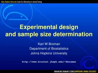
The General Situation An important issue in planning a new study is the determination of an appropriate sample size required to meet certain conditions. For example, for a study dealing with blood cholesterol levels, these conditions are typically expressed in terms such as “How large a sample do I need to be able to reject the null hypothesis that two population means are equal if the difference between them is d = 10 mg/dl?” 28 - 2
The General Approach We focus on the sample size required to test a specific hypothesis. In general, there exists a formula for calculating a sample size for the specific test statistic appropriate to test a specified hypothesis. Typically, these formulae require that the user specify the α-level and Power = (1 – β) desired, as well as the difference to be detected and the variability of the measure in question. Importantly, it is usually wise not to calculate a single number for the sample size. Rather, calculate a range of values by varying the assumptions so that you can get a sense of their impact on the resulting projected sample size. The you can pick a more suitable sample size from this range. 28 - 3
Three Common Situations In this module, we examine the process of estimating sample size for three common circumstances: 1. One-sample t-test and paired t-test, 2. Two-sample t-test, and 3. Comparison of P1 versus P2 with a z-test. The tools required for these three situations are broadly applicable and cover many of the circumstances that are typically encountered. There are sophisticated software packages that cover much more than these three and most professional biostatisticians have them readily available. 28 - 4
1. One-sample t-test and Paired t-test For testing the hypothesis: H0 : = k vs. H1 : k with a two-tailed test, the formula is: Note: this formula is used even though the test statistic could be a t-test. 28 - 5
One-Sample Example We are interested in the size for a sample from a population of blood cholesterol levels. We know that typically σ is about 30 mg/dl for these populations. The following table shows sample sizes for different levels of some of the factors included in the equation for a one sample t-test for differences between a specified population mean and the true mean. 28 - 6
One-Sample Example (contd.) α = 0.05, σ = 25, d = 5.0, Power = 0.80 28 - 7
Sample Size for One-Sample t-test Blood Cholesterol Levels: α = 0.05, σ = 25 28 - 8
2. Two Sample t-test For the hypothesis: H0: 1 = 2 vs. H1: 1 2 For a two tailed t-test, the formula is: 28 - 11
Sample Size for Testing Two tailed t-test H0: 1 = 2 vs. H1: 12 How large a sample would be needed for comparing two approaches to cholesterol lowering using α = 0.05, to detect a difference of d = 20 mg/dl or more with Power = 1- = 0.90 The formula is: Note: Textbooks do not always clearly indicate whether the formula they provide is for one group only or for both groups combined. 28 - 12
When = 30 mg/dl, β = 0.10, = 0.05; z1-/2 = 1.96 Power = 1- β ; z 1- β= 1.282 , d = 20mg/dl Hence about 50 for each group 28 - 13
3. Two-sample proportions H0 : P1 = P2 vs. H1 : P1 P2 28 - 17
Example: d = P1 - P2 = 0.7 - 0.5 = 0.2 When = 30 mg/dl, β = 0.10, = 0.05; z1-/2 = 1.96 Power = 1- β ; z1- β = 1.282 , d = 20mg/dl (P1+P2)/2 = (0.7+0.5)/2 = 0.6 Consider using N = 260, or 130 per group 28 - 18