Some Topics In Multivariate Regression
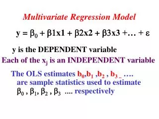
Some Topics In Multivariate Regression. Some Topics. We need to address some small topics that are often come up in multivariate regression. I will illustrate them using the Housing example. . Some Topics. Confidence intervals Scale of data Functional Form


Some Topics In Multivariate Regression
E N D
Presentation Transcript
Some Topics • We need to address some small topics that are often come up in multivariate regression. • I will illustrate them using the Housing example.
Some Topics • Confidence intervals • Scale of data • Functional Form • Tests of multi-coefficient hypotheses
Woldridgerefs to date • Chapter 1 • Chapter 2.1, 2.2,2.5 • Chapter 3.1,3.2,3.3 • Chapter 4.1, 4.2, 4.3, 4.4
Confidence Intervals (4.3) • We can construct an interval within which the true value of the parameter lies • We have seen that • P(-1.96 ≤ t ≤ 1.96)=0.95 for large N-K • More generally:
Interval b± tc *se(b) will contain b with (1-a)% confidence. • Where tc is “critical value” and is determined by the significance level (a) and the degrees of freedom (df=N-K) • For the case where N-K is large (>100) and a is 5% then tc = 1.96 • Same as the set of values of beta, which could not be rejected if they were null hypotheses • The range of possible values consistent with the data • A way of avoiding some of the ambiguity in the formulation of hypothesis tests • Formally: A procedure which will generate an interval containing the true value (1-a)% times in repeated samples
Level Option • Stata command: regress … , level(95) • Note: in assignments I want you to do it manually regress price inc_pchstock_pc if year<=1997 Source | SS df MS Number of obs = 28 -------------+------------------------------ F( 2, 25) = 88.31 Model | 1.1008e+10 2 5.5042e+09 Prob > F = 0.0000 Residual | 1.5581e+09 25 62324995.9 R-squared = 0.8760 -------------+------------------------------ Adj R-squared = 0.8661 Total | 1.2566e+10 27 465423464 Root MSE = 7894.6 ------------------------------------------------------------------------------ price | Coef. Std. Err. t P>|t| [95% Conf. Interval] -------------+---------------------------------------------------------------- inc_pc | 10.39438 1.288239 8.07 0.000 7.741204 13.04756 hstock_pc | -637054.1 174578.5 -3.65 0.001 -996605.3 -277503 _cons | 135276.6 35433.83 3.82 0.001 62299.24 208253.9 ------------------------------------------------------------------------------
Scale (2.4 & 6.1) • The scale of the data may matter • i.e. whether we measure house prices in € or €bn or even £ or $ • Exercise: try this with housing or consumption examples • Basic model: yi = b1 + b2 xi + ui
Change scale of xi : xi* = xi/c • Estimate: yi = b1* + b2* xi*+ ui • b2*= c.b2 • se(b2) = c.se(b2) • Slope coefficient and se change, all other statistics (t-stats, R2, F, etc.) unchanged.
Change scale of yi : yi* = yi/c • Estimate y*i = b1* + b2* xi + ui • b2*= b2 /c • b1*= b1 /c • se(b2) = se(b2)/c • se(b1) = se(b1)/c • t-stats, R2, F unchanged • Both X and Y rescaled yi* = yi/c, xi* = xi/c • Estimate y*i = b1* + b2* x* + ui • If rescaled by same amount: • b1*= b1 /cse(b1) = se(b1)/c • b2 and se(b2) unchanged • t-stats, R2, F unchanged
Functional Form (6.2) • Four common functional forms • Linear: qt = a + pt+ ut • Log-Log: lnqt = a + lnpt + ut • Semilog: qt = a + lnpt + ut or lnqt = a + pt + ut • How to choose? • Which fits the data best (cannot compare R2 unless y is same) • Which is most convenient (do we want elasticity, rate of return?) • How trade-off two goals
Two housing models • The level variables: marginal effects regress price inc_pchstock_pc if year<=1997 Source | SS df MS Number of obs = 28 -------------+------------------------------ F( 2, 25) = 88.31 Model | 1.1008e+10 2 5.5042e+09 Prob > F = 0.0000 Residual | 1.5581e+09 25 62324995.9 R-squared = 0.8760 -------------+------------------------------ Adj R-squared = 0.8661 Total | 1.2566e+10 27 465423464 Root MSE = 7894.6 ------------------------------------------------------------------------------ price | Coef. Std. Err. t P>|t| [95% Conf. Interval] -------------+---------------------------------------------------------------- inc_pc | 10.39438 1.288239 8.07 0.000 7.741204 13.04756 hstock_pc | -637054.1 174578.5 -3.65 0.001 -996605.3 -277503 _cons | 135276.6 35433.83 3.82 0.001 62299.24 208253.9 ------------------------------------------------------------------------------
Log on log formulation regress lpricelinclh if year<=1997 Source | SS df MS Number of obs = 28 -------------+------------------------------ F( 2, 25) = 86.21 Model | .791044208 2 .395522104 Prob > F = 0.0000 Residual | .11469849 25 .00458794 R-squared = 0.8734 -------------+------------------------------ Adj R-squared = 0.8632 Total | .905742698 27 .033546026 Root MSE = .06773 ------------------------------------------------------------------------------ lprice | Coef. Std. Err. t P>|t| [95% Conf. Interval] -------------+---------------------------------------------------------------- linc | 1.67764 .2168253 7.74 0.000 1.23108 2.1242 lh | -2.011761 .5228058 -3.85 0.001 -3.0885 -.9350227 _cons | -7.039114 2.687196 -2.62 0.015 -12.5735 -1.504731 ------------------------------------------------------------------------------
F-tests • Often we will want to test joint hypotheses • i.e. hypotheses that involve more than one coefficient • Linear restrictions • Three examples (using the log model) • H0: bH= 0 & bI= 0 H1: bH≠ 0 or bI≠0 • H0: bH= 0 & bI= 1 H1: bH≠ 0 or bI≠1 • H0: bH+bI= 1 H1: bH+bI ≠ 1
1. Test of Joint Significance • Example 1 is given the special name of “test of joint significance” • Could do K-1 t-tests, one on each of the K-1 variables • This would not be a joint hypothesis but a series of K-1 individual hypotheses • The two are not equivalent
Why Joint Hypotheses matter • Recall the sampling makes the estimators random variables • Estimators of different coefficients are correlated random variables • All the coeff are estimated from same sample in any one regression • Making statements about one coefficient implies a statement about another • Formally P(b2=0).P(b3 =0) P(b2=b3 =0)
So the set of regressions in which both are zero is smaller than the set in which either one are zero • This intuition holds for more general hypotheses.
Testing Joint Significance • As we look at all the variables it is natural to focus on the ESS • We form a test statistic • If the null hypothesis is true the ESS will be zero and RSS will be large
So we can reject the null hypothesis if the test statistic is greater than zero • How much greater? • Greater than a critical value got from the F-distribution tables with three parameters • Significance level • Df1=K-1 • Df2=N-K • The test is so useful it is reported by stata
Formal Procedure • State the Hypothesis we want to test H0: bH= 0 & bI= 0 H1: bH≠ 0 or bI≠0 • Calculate the test statistic assuming that null is true. 86.21 • Critical Value: • F(2,25)= 3.39 at 5% significance level • Stata: di invFtail(2,25,0.05) • As F>critical value we can reject the null hypothesis at the 5% signifacance level