Download
1 / 23
230 likes | 377 Views
RPC simulations for CBM. D. Gonzalez-Diaz (GSI-Darmstadt) for the CBM-TOF working group 26-02-2008. Engineering design Simulation design Detector response Physics results. 1. Engineering design. The CBM spectrometer ( di-electron /hadron setup). The CBM spectrometer ( di-muon setup).

E N D
RPC simulations for CBM D. Gonzalez-Diaz (GSI-Darmstadt) for the CBM-TOF working group 26-02-2008
Engineering design Simulation design Detector response Physics results
The CBM spectrometer (di-electron/hadron setup). The CBM spectrometer (di-muonsetup).
The CBM-ToF wall. Column and super-module layout. column Dwall = 10 m Θ[ 2.5-25 deg] 10 m Asuper-module = 1.5 m x 1 m σT = 80 ps (gaussian) 15 m
The CBM-ToF wall.Generic super-module inner structure. module honeycomb stesalit screws for rolling nylon spacers
Simulation. Module inner structure. module strip
Simulation. Wall layout. Regions of different strip length (constant width), to keep the occupancy uniform
Simulation. Number of electronic channels. • 5 different regions were defined, with 5 different cell sizes: • Padregion (1): 2.0 x 2.0 cm2 ( 27072 channels, A=11 m2 ). • Strip region (2): 2.0 x 12.5 cm2 ( 3840 x 2 channels, A=10 m2 ). • Strip region (3): 2.0 x 25.0 cm2 ( 5568 x 2 channels, A=28 m2 ). • Strip region (4): 2.0 x 50.0 cm2 ( 6150 x 2 channels, A=62 m2 ). • Strip region (5): 2.0 x 100.0 cm2 ( 2900 x 2 channels, A=58 m2 ). • TOTAL ( 63988 channels, A=170 m2 ).
Model from: A.Blanco, P. Fonte et al. NIM A, 513 (2003) 8-12 Hit generation (I). Private version. Under development. log(i) space-charge regime clusters e--I log(ithres) V=0 i = i1+ i2 + i3 no 1, t1 exponential regime gap size g V=HV i1, t1 i3, t3 i2, t2 t Separate fluctuations in avalanche multiplication, primary ionization and cluster size from deterministic multiplication in exponential regime. Assume that only multiplication inside the active region is relevant. Back-extrapolate the corresponding probability distributions for avalanche multiplication and primary ionization to t=0. Obtain from the back-extrapolated distribution of the current io, the distribution of times at threshold (time response) assuming operation in exponential regime. 2, t2 3, t3 active region xd V=0
Hit generation (II). Operative version Structure of the current TOFHitProducer! (version 1.0) particles produced locally (4 cm) are disregarded 8 gaps Vo Efficiency per gap is assumed to be 75% 2. Add gaussian fluctuations in the electronic response (independent for left and right) t1 t2 t3 t4 ...tn 1. Add gaussian fluctuations due to detector response (same for left and right) For simplicity, in this version the gaps are treated as if they were independent Prescription: the fastest hit in the left and right is stored !
NOTE: This algorithm results in a slightly non-Gaussian response (~1-2% tails towards delayed times), and is tuned to provide for particles crossing 8 gaps: σT=80 ps, σx=5 mm
Kaon identification. D. Kresan
Dynamical Fluctuations (I). D. Kresan Idea: Measure the fluctuations in the particle production, e.g.: (number of k)/(number of π), with σ= rms/mean: data2 = fin2 + exp2 +dyn2 background Experimentally: Event mixing: two tracks coming from different events mixed-events dyn2 = data2 mixed-events2
Dynamical Fluctuations (II). D. Kresan generic study (ideal tracking, no ToF segmentation, Gaussian time response) Full reconstruction dyn2 = data2 mixed-events2
Muon identification. A. Kiseleva (20/06/07) S/B ratio Efficiency % S/B ratio Efficiency % 0.3 1.6 0.13 1.8 0.11 3.5 0.05 3.8 0.008 0.8 0.002 0.9 0.095 0.2 0.014 0.2 0.005 1.4 0.001 1.6 suppression of K's and fake matches without ToF wall with ToF wall ω φ η [0.2, 0.3] ηD [0.2, 0.9] ρ
Electron identification. C. Hoehne / S. Das (29/08/07) this is where ToF works! suppression of π's
The CBM-ToF wall. Design requirements (by now). • Overall time resolutionσT ~ 80 ps. • Occupancy < 5 %for Au-Au central collisions at E=25 GeV/A. • Space resolution~ 5 mm x 5 mm. • Efficiency > 95 %. • Pile-up < 5%. • Rate capability > 20 kHz/cm2. • Reduced cross-talk and charge-sharing. • Compact and low consuming electronics (~65.000 electronic channels).
The CBM-ToF wall. Summary. Studies on fluctuations are very sensitive to the tails and to the presence of double-hits. The maximum tolerable tails and occupancy could be extracted from this observable. A better estimate of the required σT could come from a) the use of PiD in Do (or strange resonances) reconstruction, b) di-electron spectroscopy (an improvement of a factor ~2/3 will nicely overlap ToF and TRD PiD capabilities (the later very bad [a priori] below 1 GeV)) and c) K identification for flow studies, etc. Position resolution is not likely to have any constraint from physics point of view.
The CBM-ToF wall. Outlook. A detailed detector response depending on energy loss, angle, etc will be made available for physics studies in a period of 3-4 months. Debugging and comparison with data must be done first. A detailed implementation of the module inner structure requires of a concept for the electrode read-out (?) and an evaluation of the charge sharing and cross-talk in the resulting configuration. Once these studies are available the simulation design can proceed further. More physics studies are needed. CBM-ToF requirements are yet poorly constrained by physics.